Rateless Codes COS 463 Wireless Networks Lecture 10

Rateless Codes COS 463: Wireless Networks Lecture 10 Kyle Jamieson

Today 1. Rateless fountain codes – Luby Transform (LT) Encoding – LT Decoding 2. Rateless Spinal codes 2

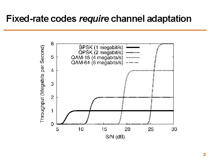
Fixed-rate codes require channel adaptation 3

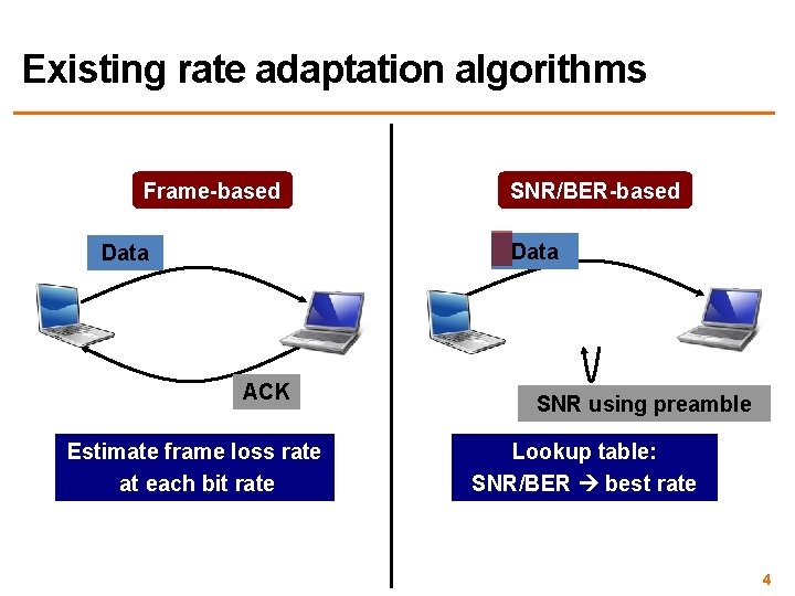
Existing rate adaptation algorithms Frame-based SNR/BER-based Data ACK Estimate frame loss rate at each bit rate SNR using preamble Lookup table: SNR/BER best rate 4

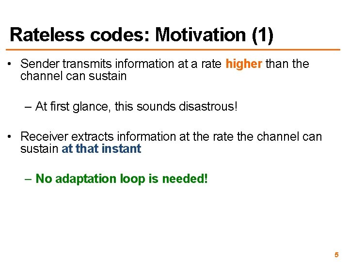
Rateless codes: Motivation (1) • Sender transmits information at a rate higher than the channel can sustain – At first glance, this sounds disastrous! • Receiver extracts information at the rate the channel can sustain at that instant – No adaptation loop is needed! 5

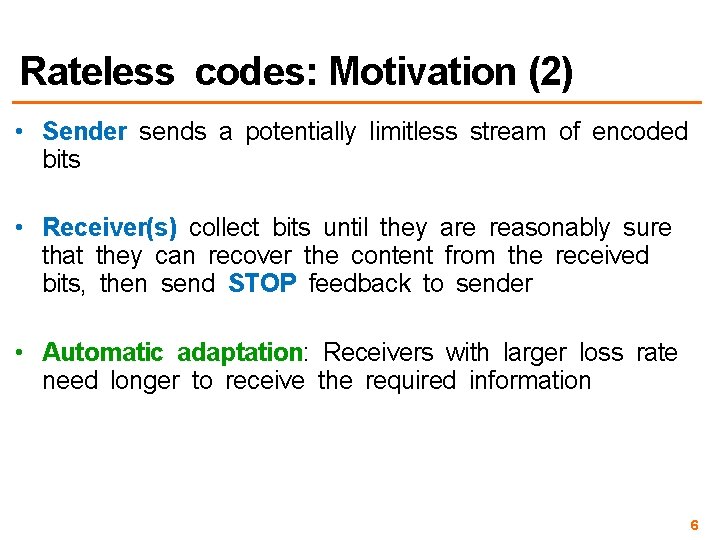
Rateless codes: Motivation (2) • Sender sends a potentially limitless stream of encoded bits • Receiver(s) collect bits until they are reasonably sure that they can recover the content from the received bits, then send STOP feedback to sender • Automatic adaptation: Receivers with larger loss rate need longer to receive the required information 6

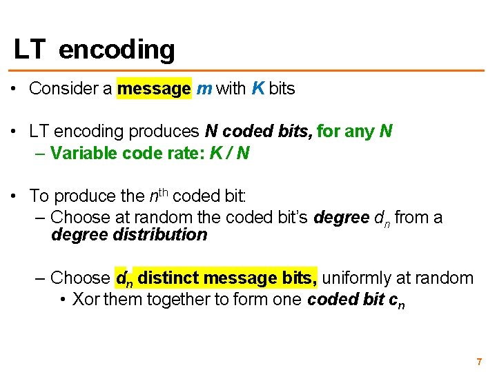
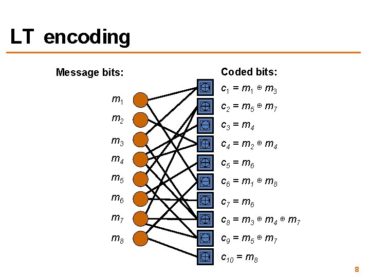
LT encoding • Consider a message m with K bits • LT encoding produces N coded bits, for any N – Variable code rate: K / N • To produce the nth coded bit: – Choose at random the coded bit’s degree dn from a degree distribution – Choose dn distinct message bits, uniformly at random • Xor them together to form one coded bit cn 7

LT encoding Message bits: m 1 m 2 Coded bits: c 1 = m 1 ⊕ m 3 c 2 = m 5 ⊕ m 7 c 3 = m 4 m 3 c 4 = m 2 ⊕ m 4 c 5 = m 6 m 5 c 6 = m 1 ⊕ m 8 m 6 c 7 = m 6 m 7 c 8 = m 3 ⊕ m 4 ⊕ m 7 m 8 c 9 = m 5 ⊕ m 7 c 10 = m 8 8

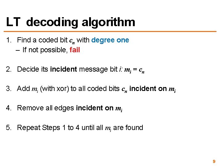
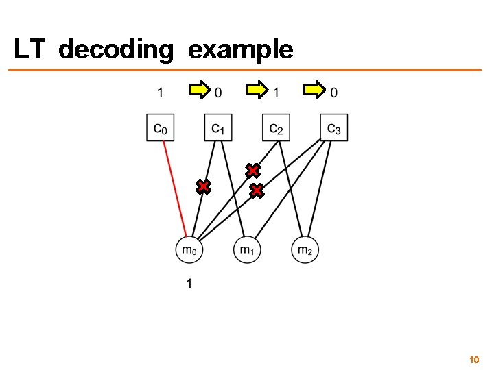
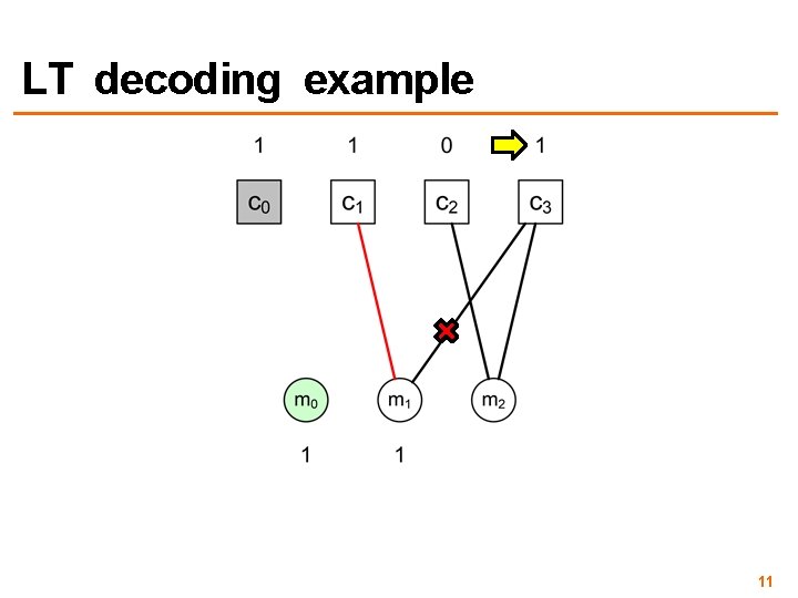
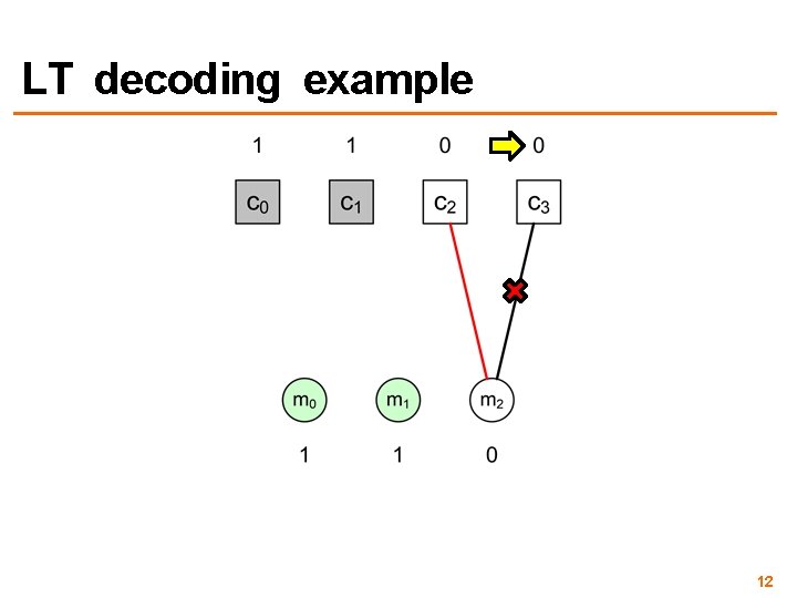
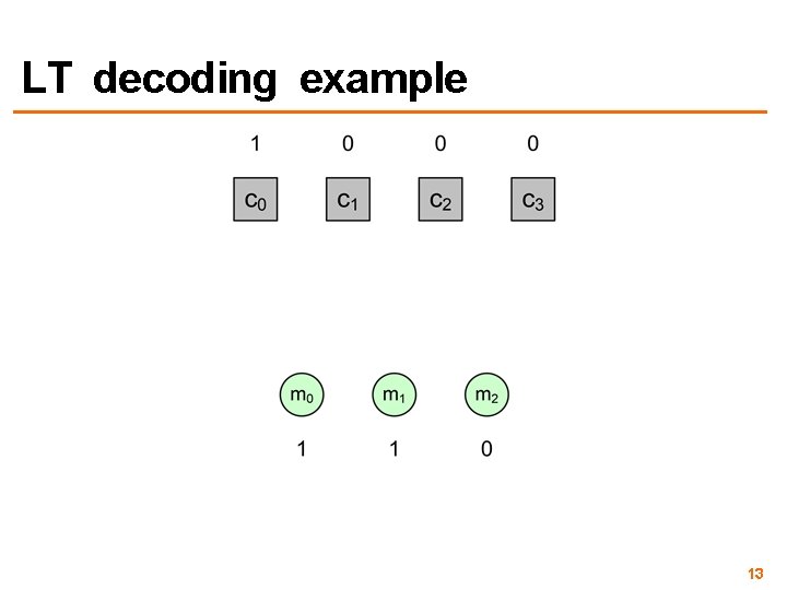
LT decoding algorithm 1. Find a coded bit cn with degree one – If not possible, fail 2. Decide its incident message bit i: mi = cn 3. Add mi (with xor) to all coded bits cn incident on mi 4. Remove all edges incident on mi 5. Repeat Steps 1 to 4 until all mi are found 9

LT decoding example 10

LT decoding example 11

LT decoding example 12

LT decoding example 13

Today 1. Rateless fountain codes – Luby Transform (LT) Encoding – LT Decoding 2. Rateless Spinal codes – Encoding Spinal Codes – Decoding Spinal codes – Performance evaluation 14

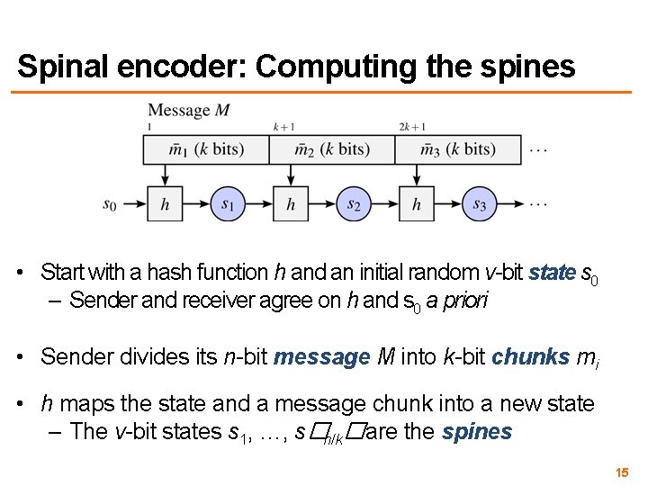
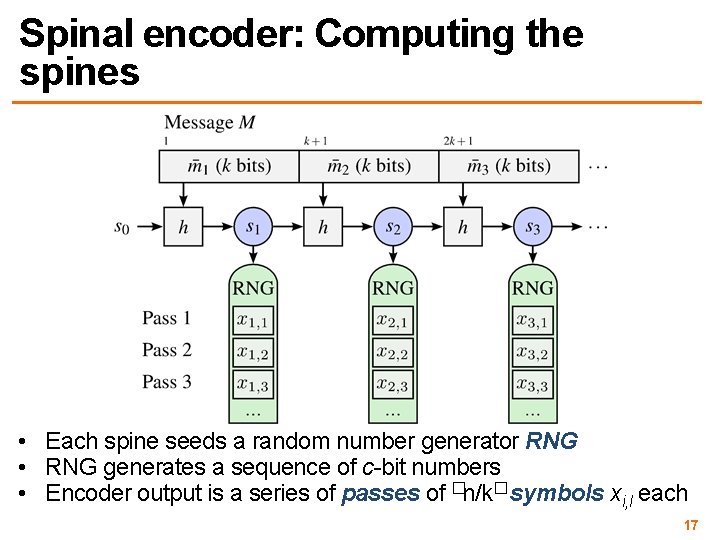
Spinal encoder: Computing the spines • Start with a hash function h and an initial random v-bit state s 0 – Sender and receiver agree on h and s 0 a priori • Sender divides its n-bit message M into k-bit chunks mi • h maps the state and a message chunk into a new state – The v-bit states s 1, …, s�n/k�are the spines 15

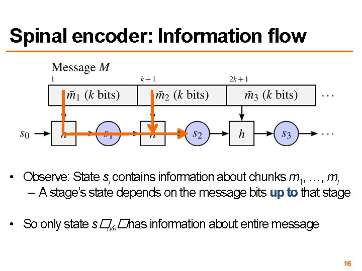
Spinal encoder: Information flow • Observe: State si contains information about chunks m 1, …, mi – A stage’s state depends on the message bits up to that stage • So only state s�n/k�has information about entire message 16

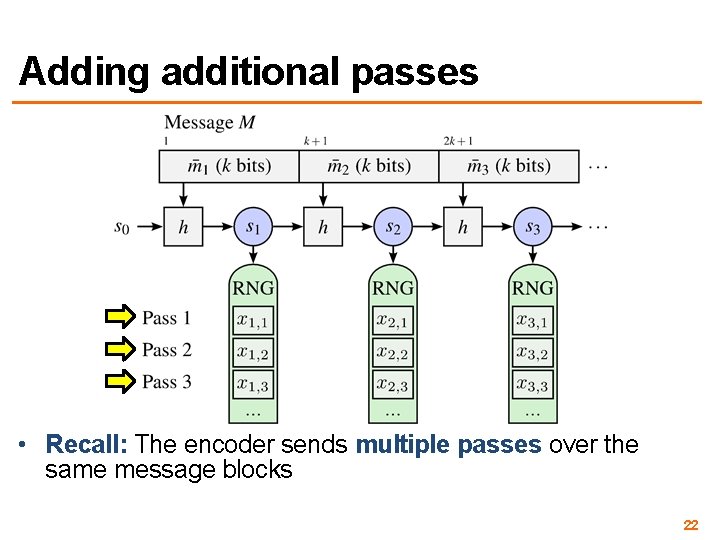
Spinal encoder: Computing the spines • Each spine seeds a random number generator RNG • RNG generates a sequence of c-bit numbers • Encoder output is a series of passes of �n/k� symbols xi, l each 17

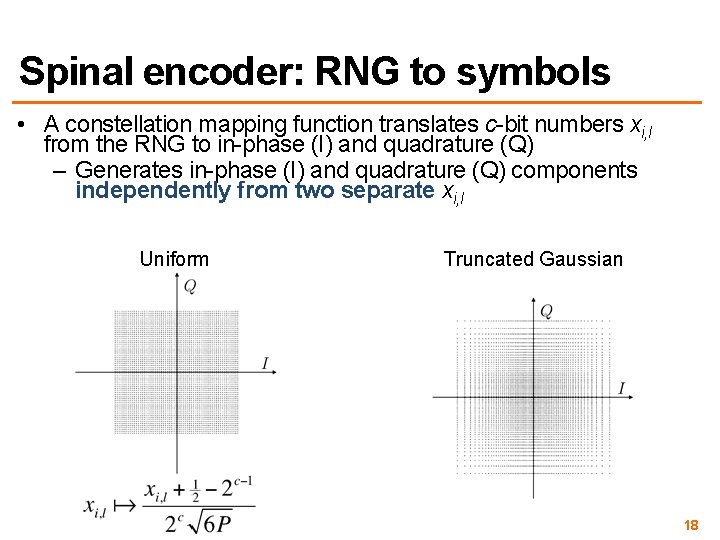
Spinal encoder: RNG to symbols • A constellation mapping function translates c-bit numbers xi, l from the RNG to in-phase (I) and quadrature (Q) – Generates in-phase (I) and quadrature (Q) components independently from two separate xi, l Uniform Truncated Gaussian 18

Today 1. Rateless fountain codes – Luby Transform (LT) Encoding – LT Decoding 2. Rateless Spinal codes – Encoding Spinal Codes – Decoding Spinal codes – “Maximum-likelihood” decoding – The Bubble Decoder – Puncturing for higher rate – Performance evaluation 19

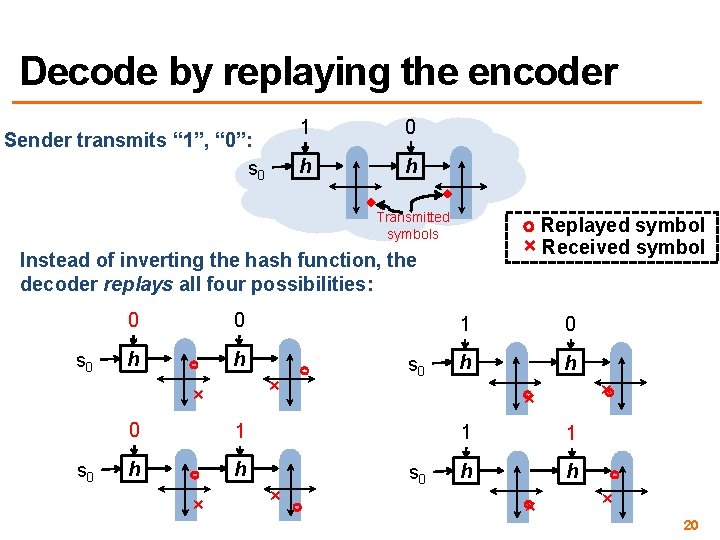
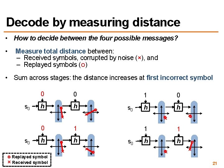
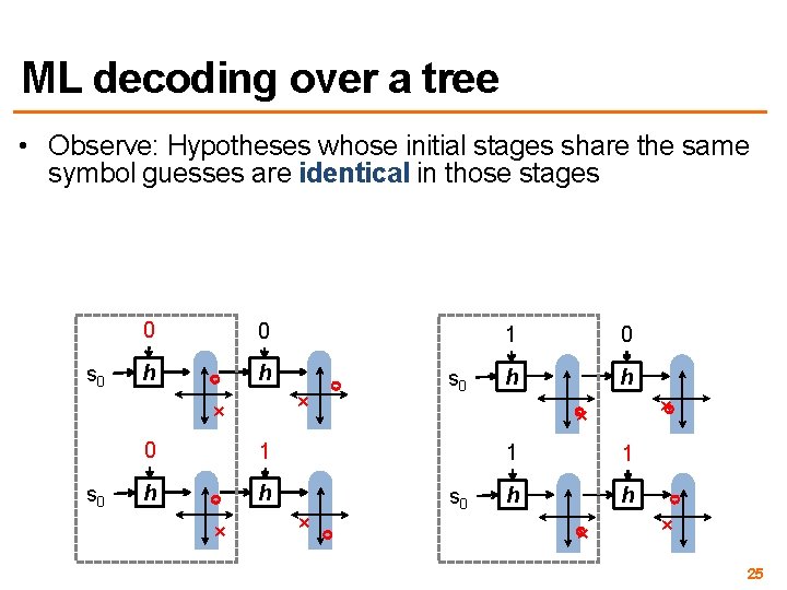
Decode by replaying the encoder Sender transmits “ 1”, “ 0”: s 0 1 0 h h Transmitted symbols Replayed symbol × Received symbol Instead of inverting the hash function, the decoder replays all four possibilities: 0 s 0 h 0 h × × 0 s 0 h s 0 × h h × × h × 0 1 1 s 0 1 1 h h × × 20

Decode by measuring distance • How to decide between the four possible messages? • Measure total distance between: – Received symbols, corrupted by noise (×), and – Replayed symbols ( ) • Sum across stages: the distance increases at first incorrect symbol 0 s 0 h 0 h × × 0 s 0 h Replayed symbol × Received symbol s 0 × h h × × h × 0 1 1 s 0 1 1 h h × × 21

Adding additional passes • Recall: The encoder sends multiple passes over the same message blocks 22

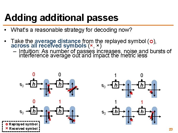
Adding additional passes • What’s a reasonable strategy for decoding now? • Take the average distance from the replayed symbol ( ), across all received symbols (×, ×) – Intuition: As number of passes increases, noise and bursts of interference average out and impact the metric less 0 h 0 h ×× ×× 0 s 0 h Replayed symbol × Received symbol s 0 ×× h ×× 0 h h × × 1 1 s 0 1 1 h h × × ×× 23

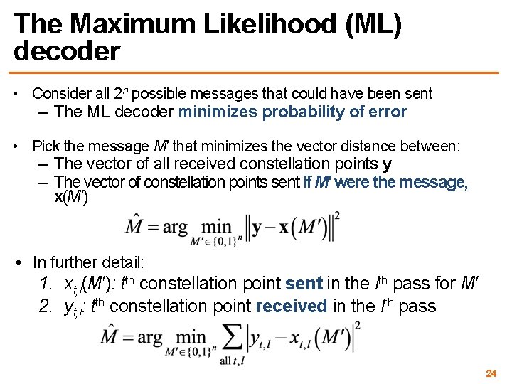
The Maximum Likelihood (ML) decoder • Consider all 2 n possible messages that could have been sent – The ML decoder minimizes probability of error • Pick the message M′ that minimizes the vector distance between: – The vector of all received constellation points y – The vector of constellation points sent if M′ were the message, x(M′) • In further detail: 1. xt, l(M′): tth constellation point sent in the lth pass for M′ 2. yt, l: tth constellation point received in the lth pass 24

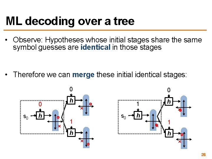
ML decoding over a tree • Observe: Hypotheses whose initial stages share the same symbol guesses are identical in those stages 0 h 0 h × × 0 s 0 h s 0 × h h × × h × 0 1 1 s 0 1 1 h h × × 25

ML decoding over a tree • Observe: Hypotheses whose initial stages share the same symbol guesses are identical in those stages • Therefore we can merge these initial identical stages: 0 h 0 s 0 h 0 × × s 0 1 h 1 × h × h 1 h × × 26

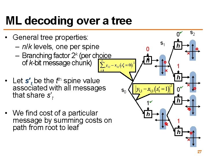
ML decoding over a tree • General tree properties: – n/k levels, one per spine – Branching factor 2 k (per choice of k-bit message chunk) 0 h s 1 tth • We find cost of a particular message by summing costs on path from root to leaf h × × • Let s′t be the spine value associated with all messages that share s′t s 2 ✔ 0 1 h ✔ 0 s 0 × h 1✔ × h × 1 h × 27

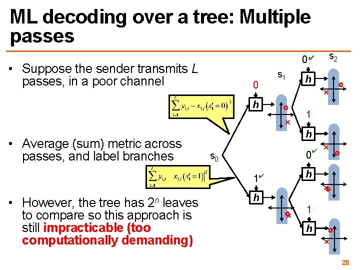
ML decoding over a tree: Multiple passes • Suppose the sender transmits L passes, in a poor channel 0 h s 1 h 0 s 0 1 ✔ × h 1✔ • However, the tree has 2 n leaves to compare so this approach is still impracticable (too computationally demanding) h × × • Average (sum) metric across passes, and label branches s 2 0✔ × h × 1 h × 28

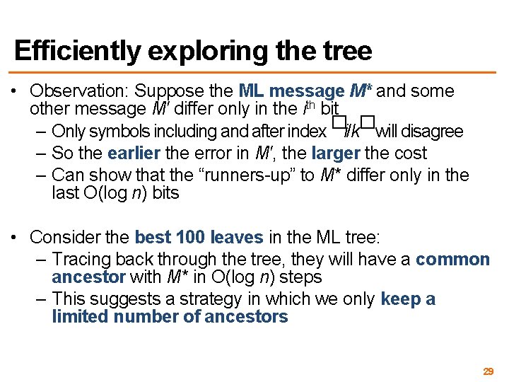
Efficiently exploring the tree • Observation: Suppose the ML message M* and some other message M′ differ only in the ith bit – Only symbols including and after index �i/k�will disagree – So the earlier the error in M′, the larger the cost – Can show that the “runners-up” to M* differ only in the last O(log n) bits • Consider the best 100 leaves in the ML tree: – Tracing back through the tree, they will have a common ancestor with M* in O(log n) steps – This suggests a strategy in which we only keep a limited number of ancestors 29

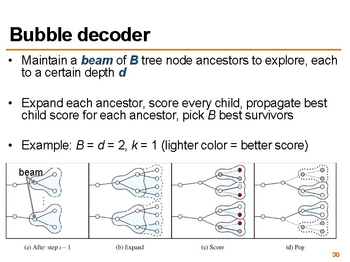
Bubble decoder • Maintain a beam of B tree node ancestors to explore, each to a certain depth d • Expand each ancestor, score every child, propagate best child score for each ancestor, pick B best survivors • Example: B = d = 2, k = 1 (lighter color = better score) beam 30

Decoding complexity • The bubble decoder operates in n/k − d steps – Each step explores B∙ 2 kd nodes, evaluating the RNG L times – Selecting the best B candidates takes B∙ 2 k comparisons • Overall cost: O((n/k)BL∙ 2 kd) hashes, O((n/k)B∙ 2 k) comparisons • Comparison with LDPC belief propagation algorithms – These operate in iterations, too, involve all message bits – But, these are also quite parallelizable – Hard to give exact head-to-head comparison 31

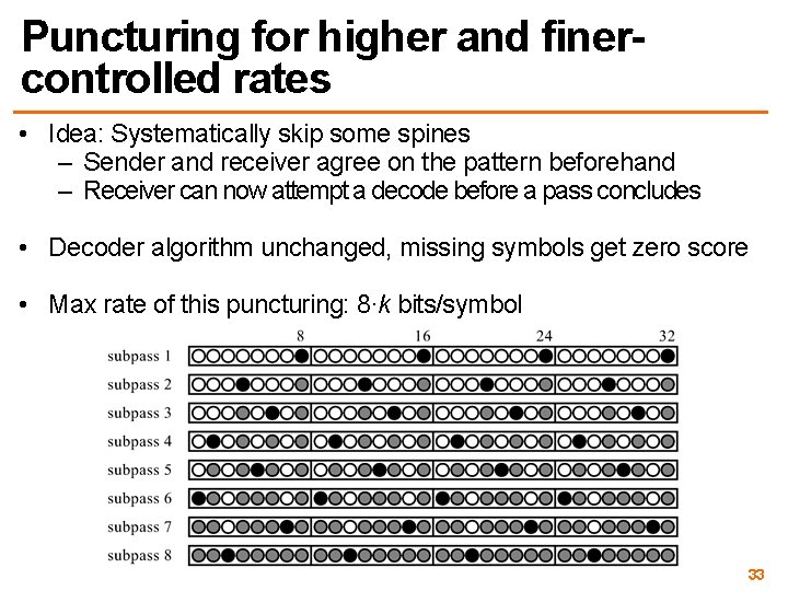
Adjusting the rate • Spinal codes as described so far uses different numbers of passes to adjust the rate • Two problems in Spinal codes as described so far: 1. Must transmit one full pass, so max out at k bits/symbol • Increase k? No: Decoding cost is exponential in k 1. Sending L passes reduces rate to k/L—abrupt drop • Introduces plateaus in the rate versus SNR curve 32

Puncturing for higher and finercontrolled rates • Idea: Systematically skip some spines – Sender and receiver agree on the pattern beforehand – Receiver can now attempt a decode before a pass concludes • Decoder algorithm unchanged, missing symbols get zero score • Max rate of this puncturing: 8∙k bits/symbol 33

Framing at the link layer • Sender and receiver need to maintain synchronization – Sender uses a short sequence number protected by a highly redundant code • Unusual property of Spinal codes: Shorter message length n is more efficient – This is in opposition to the trend most codes follow – Divide the link-layer frame into shorter checksumprotected code blocks • If half-duplex radio, when should sender wait for feedback? – For more information, see Rate. More (Mobi. Com ‘ 12) 34

Today 1. Rateless fountain codes – Luby Transform (LT) Encoding – LT Decoding 2. Rateless Spinal codes – Encoding Spinal Codes – Decoding Spinal codes – Performance evaluation 35

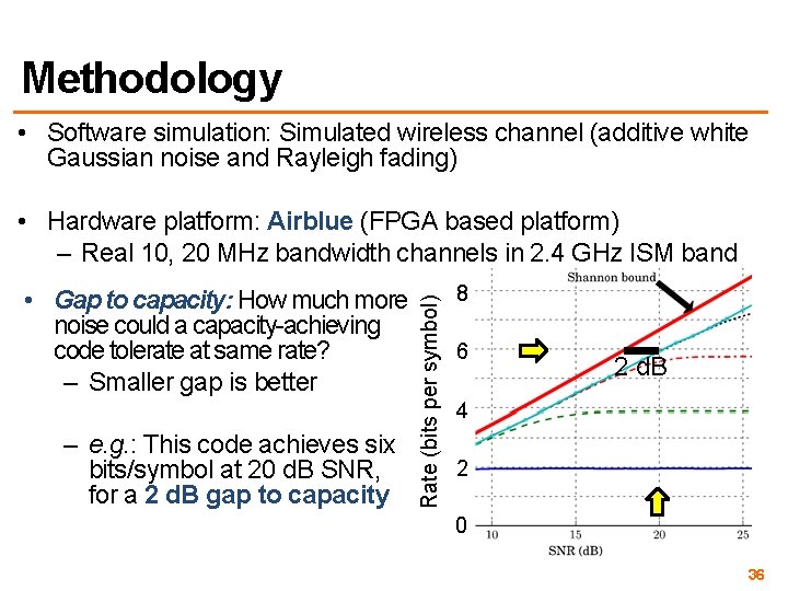
Methodology • Software simulation: Simulated wireless channel (additive white Gaussian noise and Rayleigh fading) • Gap to capacity: How much more noise could a capacity-achieving code tolerate at same rate? – Smaller gap is better – e. g. : This code achieves six bits/symbol at 20 d. B SNR, for a 2 d. B gap to capacity Rate (bits per symbol) • Hardware platform: Airblue (FPGA based platform) – Real 10, 20 MHz bandwidth channels in 2. 4 GHz ISM band 8 6 2 d. B 4 2 0 36

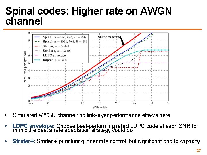
Spinal codes: Higher rate on AWGN channel • Simulated AWGN channel: no link-layer performance effects here • LDPC envelope: Choose best-performing rated LDPC code at each SNR to mimic the best a rate adaptation strategy could do • Strider+: Strider + puncturing: finer rate control, but significant gap to capacity 37

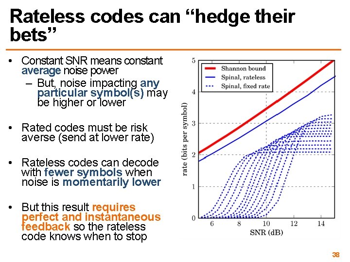
Rateless codes can “hedge their bets” • Constant SNR means constant average noise power – But, noise impacting any particular symbol(s) may be higher or lower • Rated codes must be risk averse (send at lower rate) • Rateless codes can decode with fewer symbols when noise is momentarily lower • But this result requires perfect and instantaneous feedback so the rateless code knows when to stop 38

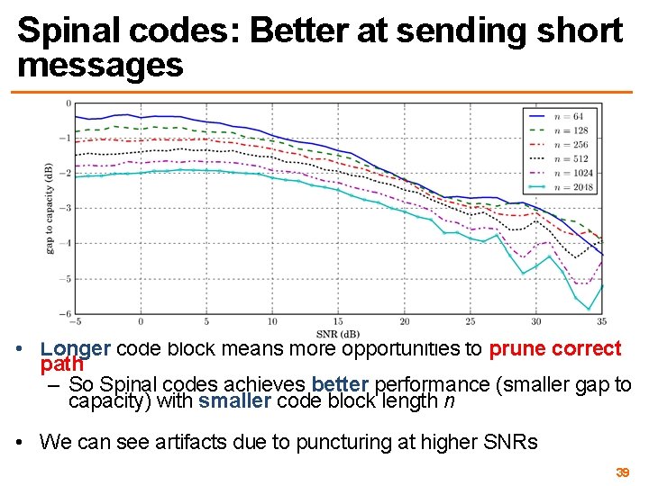
Spinal codes: Better at sending short messages • Longer code block means more opportunities to prune correct path – So Spinal codes achieves better performance (smaller gap to capacity) with smaller code block length n • We can see artifacts due to puncturing at higher SNRs 39

Spinal Codes: Conclusion • Spinal Codes give performance close to Shannon capacity • Eliminate the need to run a bit rate adaptation algorithm • Simpler design and better performance • Link layer design more open, incurs overhead between transmissions 40

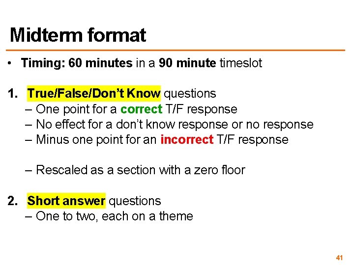
Midterm format • Timing: 60 minutes in a 90 minute timeslot 1. True/False/Don’t Know questions – One point for a correct T/F response – No effect for a don’t know response or no response – Minus one point for an incorrect T/F response – Rescaled as a section with a zero floor 2. Short answer questions – One to two, each on a theme 41

Friday Precept: Midterm Review Tuesday Topic: Signals and Systems Preliminaries Next Thursday: In-Class Midterm 42