Rapid and Accurate Calculation of the Voigt Function

Rapid and Accurate Calculation of the Voigt Function Kendra L. Letchworth D. Chris Benner 61 st International Symposium on Molecular Spectroscopy June 20, 2006

Outline • • • Overview Mathematical Approximations Programming Techniques Accuracy Comparisons Speed Comparisons

Overview • Spectra with higher signal to noise ratios require more accurate analysis routines. • Most fitting programs and simulations perform millions of calculations, so routines must also be fast. • Our routine calculates the Voigt profile to a relative accuracy of 10 -6. • 100 times more accurate than routines such as Drayson & Humlíček. • However, it requires less calculation time than those same routines.

The Voigt Profile • • • v - v 0 : distance from line center αL : Lorentz half-width αD : Doppler half-width

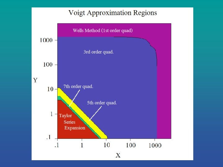
Mathematical Approximations: Gauss-Hermite Quadrature Points - vi Quadrature Weights - wi Real Part: Imaginary Part: Expression simplified using: • Symmetry • Odd-order quadrature • Repeating expressions within equations

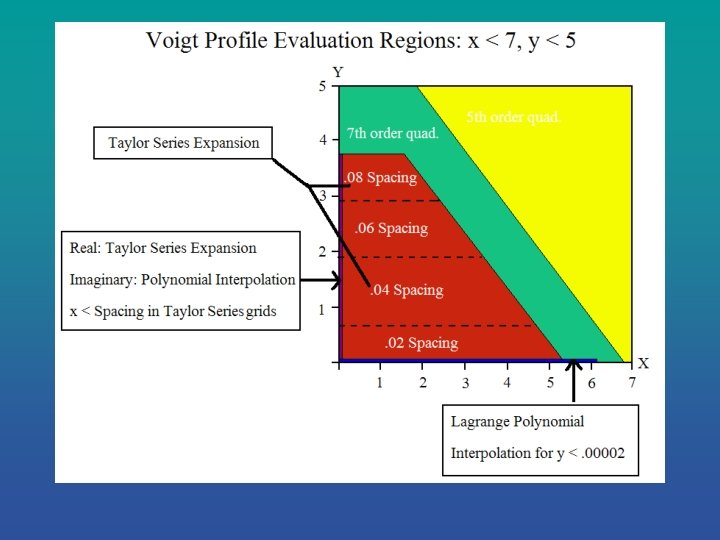
Mathematical Approximations: Taylor Series Expansion • Uses table of pre-computed values of the complex Voigt function (K+i. L) and its derivatives. • Evaluation formula for real part (3 rd order Taylor expansion) • Δx=x-x 0, Δy=y-y 0 where (x 0, y 0) is the closest gridpoint. • ∂2 K/∂x 2=-∂2 K/∂y 2 decreases the number of stored derivatives of the real part (K) from 9 to 6.

• Derivatives of the imaginary part (L) can be represented as functions of the derivatives of the real part since ∂L/∂x=-∂K/∂y and ∂L/∂y=∂K/∂x. • Evaluation formula for imaginary part: • A total of 8 values must be stored for each grid point (x 0, y 0) : K, L, ∂K/∂x, ∂K/∂y, ∂2 K/∂x 2, ∂3 K/∂x 3, ∂3 K/∂y 3.

Mathematical Approximations: Lagrange Interpolating Polynomials • Used only in small areas when other methods fail. • Employ equal grid point spacing dx and dy. • v 1, v 2, v 3 are three grid points and ∆v=(v- v 2)/dv • Four polynomial interpolations of P(v) below are required for a spline interpolation of real or imaginary part.

Programming Techniques • Calculates the Voigt profile for an entire spectral line at one time, removing unnecessary subroutine calls. • Each parameter involving y is calculated only once per spectral line, saving calculation time. • To do this we require equal spacing in wavenumber; a version of the routine called for individual points is available, but not as time efficient. • Interpolation tables stored as binary files on the hard drive and read in only when needed. • All files take up a total of 1. 5 MB of memory, a small price to pay for the increase in accuracy and speed.

Accuracy Comparisons: Real Less than 10 -4 ↓ ↑ Less than 10 -6

Routines calculating only the Real Part Maximum Error 7 x 10 -4 Maximum Error 1. 5 x 10 -2 How bad do some routines get at small y?

Accuracy Comparisons: Imaginary Relative Error in Imaginary Voigt- Benner & Letchworth Less than 10 -4 ↓ ↑ Less than 10 -6 Relative Error in Imaginary Voigt - Humlíček

Speed Comparisons Humlíček

Time Trials for Benner & Letchworth Time Trials for Humlíček (vectorized)

Humlíček * Note that the “non-vectorized” version of Benner & Letchworth is just the vectorized version, called only for one point (x, y), thus it contains a large amount of code which could be removed to boost speed. ** These times are close to the final values, but the routine with derivatives is still undergoing final testing.

Conclusions • Our Voigt routine provides accuracy without losing time, includes the imaginary part of the function for applications to line-mixing, and in most places is considerably faster than routines like Drayson & Humlíček. • Option of returning the derivatives of the real Voigt profile with respect to x and y: -Approximately < 10 -3 relative accuracy -some additional calculation time required. • The accuracy provided by this routine is becoming necessary as spectra become better.

References • • B. H. Armstrong, J. Q. S. R. T. , Vol. 7, 1966. S. R. Drayson, J. Q. S. R. T. , Vol. 16, 1976. J. H. Pierluissi, J. Q. S. R. T. , Vol. 18, 1977. Twitty, Rarig, & Thompson, J. Q. S. R. T. , Vol. 24, 1980. J. Humlíček, J. Q. S. R. T. , Vol. 27, 1982. F. Schreier, J. Q. S. R. T. , Vol. 48, 1992. R. J. Wells, J. Q. S. R. T. , Vol. 62, 1999.