RandomVariate Generation Andy Wang CIS 5930 03 Computer

Random-Variate Generation Andy Wang CIS 5930 -03 Computer Systems Performance Analysis

Random-Variate Generation • Methods to generate nonuniform variables – Each method is applicable to a subset of the distribution – For a distribution, one method may be more efficient than the others 2

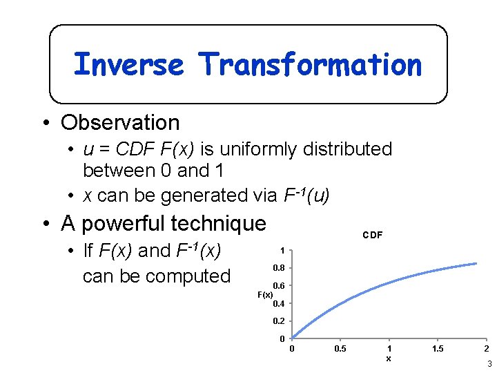
Inverse Transformation • Observation • u = CDF F(x) is uniformly distributed between 0 and 1 • x can be generated via F-1(u) • A powerful technique • If F(x) and F-1(x) can be computed CDF 1 0. 8 F(x) 0. 6 0. 4 0. 2 0 0 0. 5 1 x 1. 5 2 3

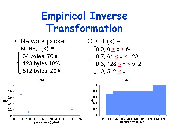
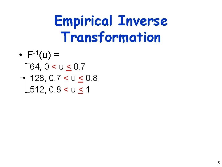
Empirical Inverse Transformation • Network packet sizes, f(x) = CDF F(x) = 0. 0, 0 < x < 64 0. 7, 64 < x < 128 0. 8, 128 < x < 512 1. 0, 512 < x 64 bytes, 70% 128 bytes, 10% 512 bytes, 20% CDF PMF 1 1 0. 8 0. 6 f(x) 0. 4 F(x) 0. 6 0. 4 0. 2 0 0 0 64 128 192 256 320 384 448 512 576 packet size (bytes) 4

Empirical Inverse Transformation • F-1(u) = 64, 0 < u < 0. 7 128, 0. 7 < u < 0. 8 512, 0. 8 < u < 1 5

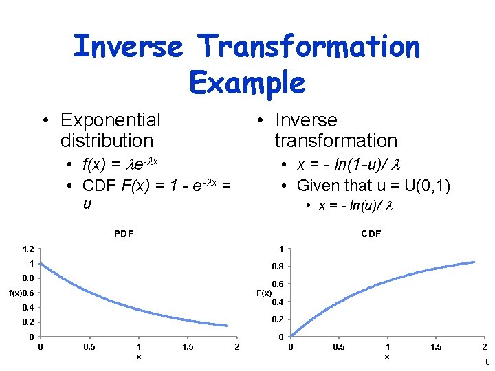
Inverse Transformation Example • Exponential distribution • Inverse transformation • f(x) = e- x • CDF F(x) = 1 - e- x = u • x = - ln(1 -u)/ • Given that u = U(0, 1) • x = - ln(u)/ PDF CDF 1. 2 1 1 0. 8 f(x)0. 6 F(x) 0. 4 0. 6 0. 4 0. 2 0 0. 5 1 x 1. 5 2 6

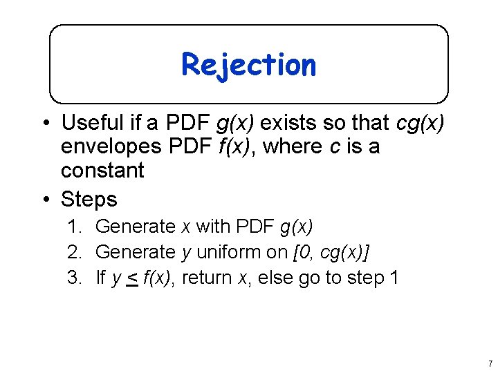
Rejection • Useful if a PDF g(x) exists so that cg(x) envelopes PDF f(x), where c is a constant • Steps 1. Generate x with PDF g(x) 2. Generate y uniform on [0, cg(x)] 3. If y < f(x), return x, else go to step 1 7

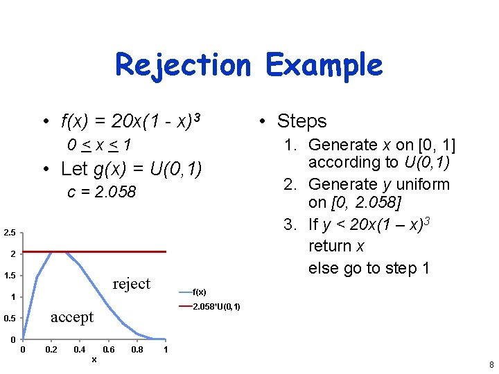
Rejection Example • f(x) = 20 x(1 - x)3 0<x<1 • Let g(x) = U(0, 1) c = 2. 058 2. 5 2 1. 5 reject 1. Generate x on [0, 1] according to U(0, 1) 2. Generate y uniform on [0, 2. 058] 3. If y < 20 x(1 – x)3 return x else go to step 1 f(x) 1 2. 058*U(0, 1) accept 0. 5 • Steps 0 0 0. 2 0. 4 0. 6 x 0. 8 1 8

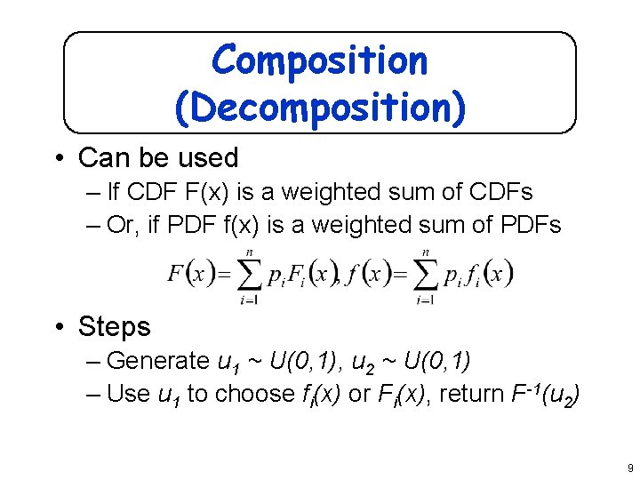
Composition (Decomposition) • Can be used – If CDF F(x) is a weighted sum of CDFs – Or, if PDF f(x) is a weighted sum of PDFs • Steps – Generate u 1 ~ U(0, 1), u 2 ~ U(0, 1) – Use u 1 to choose fi(x) or Fi(x), return F-1(u 2) 9

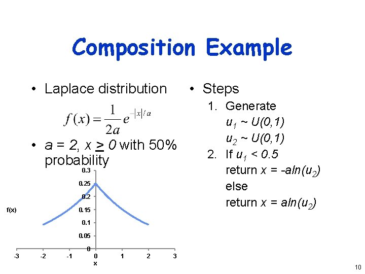
Composition Example • Laplace distribution • Steps • a = 2, x > 0 with 50% probability 0. 3 0. 25 0. 2 f(x) 0. 15 1. Generate u 1 ~ U(0, 1) u 2 ~ U(0, 1) 2. If u 1 < 0. 5 return x = -aln(u 2) else return x = aln(u 2) 0. 1 0. 05 0 -3 -2 -1 0 x 1 2 3 10

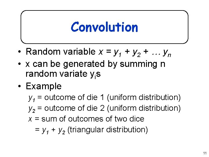
Convolution • Random variable x = y 1 + y 2 + … yn • x can be generated by summing n random variate yis • Example y 1 = outcome of die 1 (uniform distribution) y 2 = outcome of die 2 (uniform distribution) x = sum of outcomes of two dice = y 1 + y 2 (triangular distribution) 11

Choosing Random-Variate Generation Techniques • Use inversion if CDF is invertible • Use composition if CDF/PDF sum of other CDFs/PDFs • Use convolution if the variate a sum of other variates • Use rejection if a bounding PDF function exists • Use empirical inversion as needed 12

White Slide 13