Randomized Planning for Short Inspection Paths Tim Danner

Randomized Planning for Short Inspection Paths Tim Danner Lydia E. Kavraki Department of Computer Science Rice University

Outline • • Introduction Art Gallery and Watchman Route Problems Adding Realism 2 -D Algorithm – Selecting Guards – Connecting Guards – Results • 3 -D Algorithm – Differences – Preliminary Results • Future Work

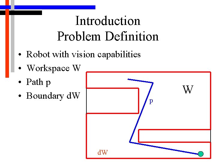
Introduction Problem Definition • • Robot with vision capabilities Workspace W Path p Boundary d. W p W

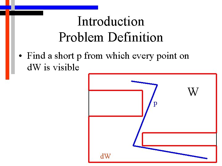
Introduction Problem Definition • Find a short p from which every point on d. W is visible p d. W W

Introduction Uses • Autonomous inspection of spacecraft exterior • Flying camera building inspection • Virtual reality architecture walkthrough

Art Gallery Problem • Find minimal number of positions for guards to stand so that every point in a gallery is “visible” to at least one guard • “Visible” is defined as the line of sight between the guard and the point lies entirely in W

Watchman Route Problem • For workspace W, find the shortest path p in W such that every point on the boundary d. W can be seen by a point on path p

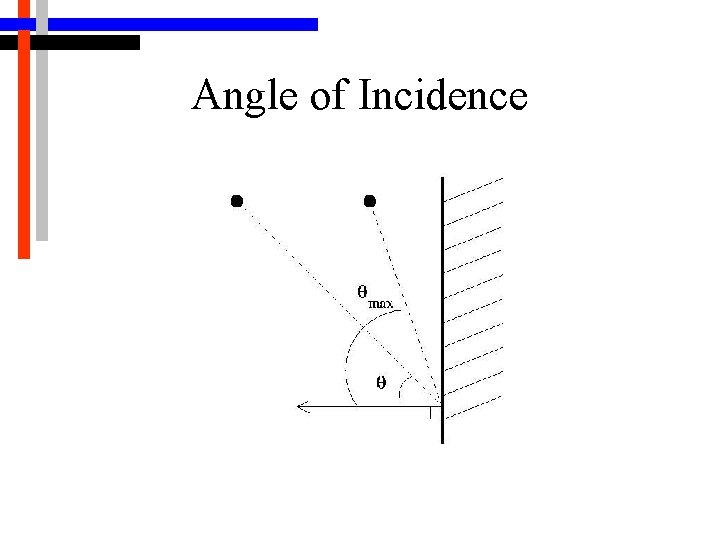
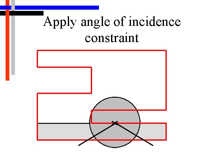
Adding Realism • “Straight-line” visibility is not very realistic for real sensors • Length of line of sight must have a maximum • Angle of incidence of line of sight must have a maximum – 60 degrees is a typical value • System is adaptable for different sensors • 2 -D vs 3 -D

Angle of Incidence

2 -D Algorithm • Sensing with real sensors is time consuming • Two parts to the algorithm: – Solve “art gallery problem” to find locations for sensing locations - “guards” – Connect the guards with a short path, the “watchman route”

2 -D Algorithm Selecting the Guards • True minimal set of guards is an NP-hard problem • Randomized planner is used in this case • Uses Gonzalez-Banos and Latombe’s randomized, incremental algorithm

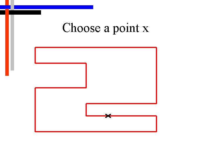
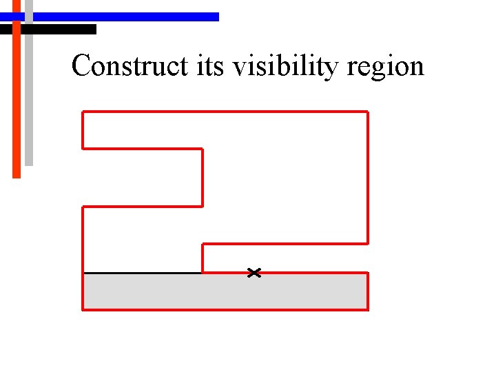
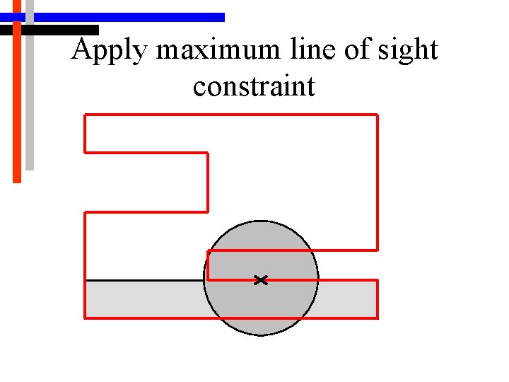
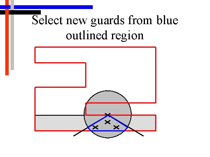
2 -D Algorithm Selecting the Guards • Main structure is a loop • At each iteration, a point x on the border d. W of W that is not yet guarded is chosen randomly • Construct region which can see x (same as region which x can see) • Apply two range constraints: limited length line of sight and angle of incidence

Choose a point x

Construct its visibility region

Apply maximum line of sight constraint

Apply angle of incidence constraint

Select new guards from blue outlined region

2 -D Algorithm Selecting the Guards • Sample region k times, evaluating each point as a possible new guard • Sample which can cover the largest portion of the new length of border is chosen as the new guard and guarded border is updated • Loop repeats until the entire border is guarded

2 -D Algorithm Selecting the Guards • One problematic case is sharp interior angles • A “disproportionately large” number of guards may be needed and hard to place • Incremental loop can be terminated

2 -D Algorithm Connecting the Guards • Basically, find an order to connect guards out of a possible n! orders • Connect guards using a graph algorithm • In this manner, the problem becomes a “traveling salesman problem”

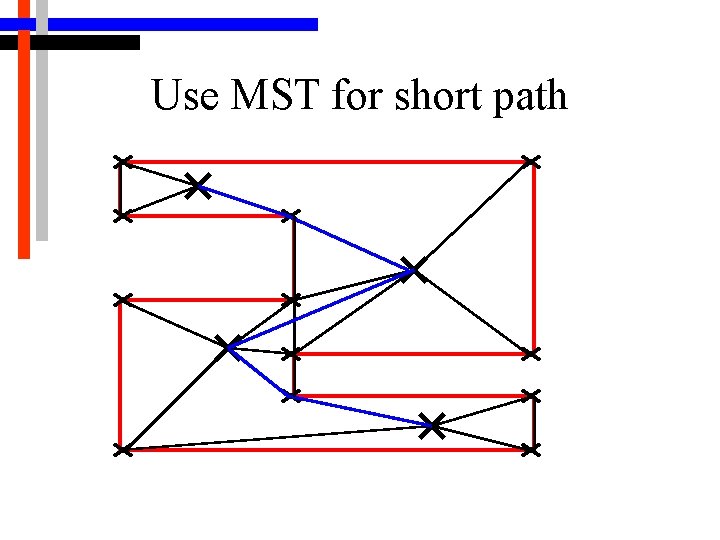
2 -D Algorithm Connecting the Guards • Actually use an approximation to the TSP – preorder walk of a Minimum Spanning Tree • Applies in cases where the triangle inequality holds, which is the case for graphs in R 2 and R 3 (which our graph of guards is) • Path length is bounded by 2 X actual TSP for complete graphs • If workspace is connected, then the graph is complete (for an inspection path to exist, the space must be connected)

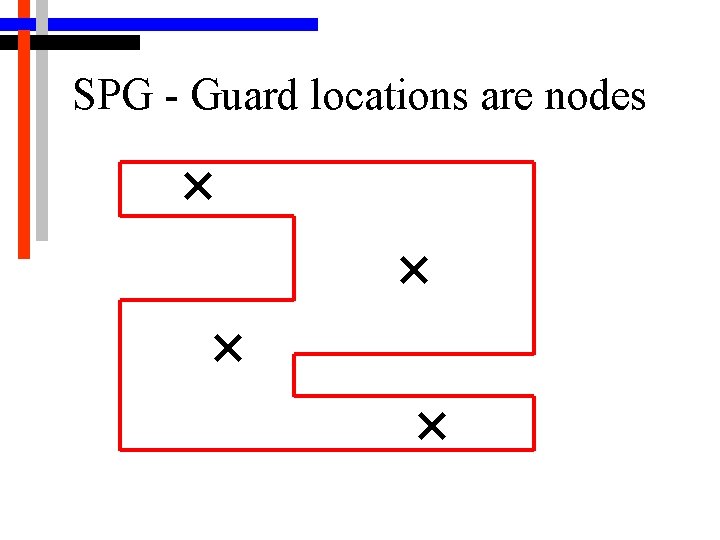
2 -D Algorithm Connecting the Guards • Shortest Paths Graph (SPG) – One node for each guard – One edge for each pair of guards – Weight is assigned to each edge (i, j) that is equal to the shortest collision-free path from point i to j – May be straight line or more complex

SPG - Guard locations are nodes

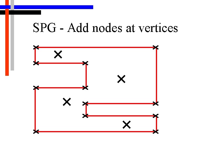
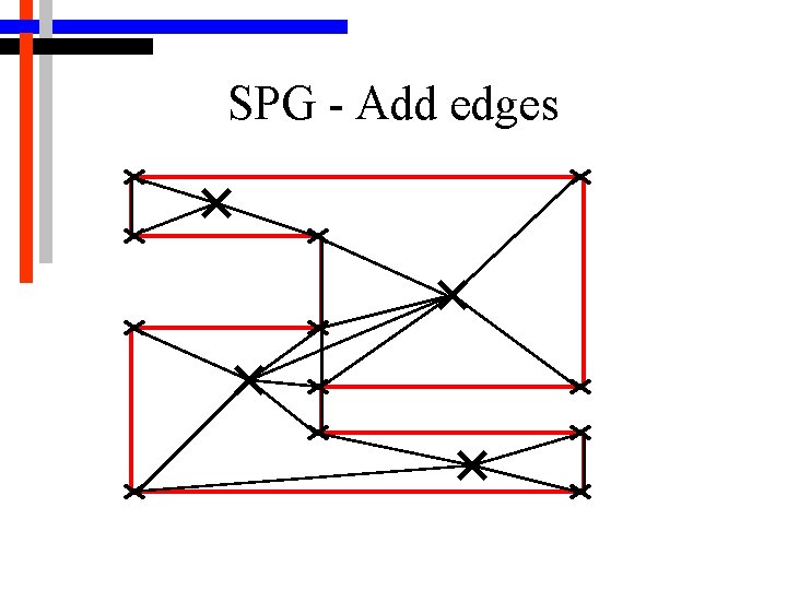
2 -D Algorithm Connecting the Guards • Shortest path between two points is done by constructing and searching another graph, the workspace-guard roadmap • Workspace-guard roadmap has one node for each vertex on d. W and one node for each guard • Has an edge between a pair of nodes i and j if and only if it is collision-free

SPG - Add nodes at vertices

SPG - Add edges

Use MST for short path

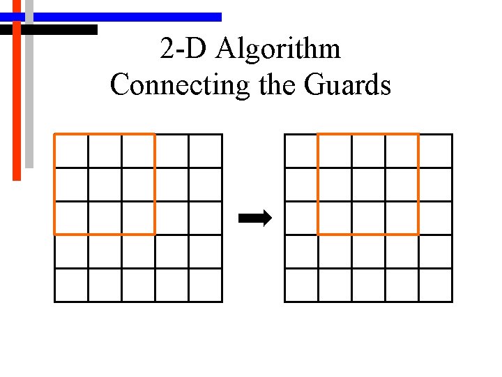
2 -D Algorithm Connecting the Guards • Complete graph has n 2 edges, but we can use a shortcut • Only connect close points, by dividing workspace into rectangular grid • About 10 nodes per cell • Connection is made with a moving 3 X 3 window

2 -D Algorithm Connecting the Guards

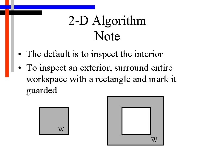
2 -D Algorithm Note • The default is to inspect the interior • To inspect an exterior, surround entire workspace with a rectangle and mark it guarded W W

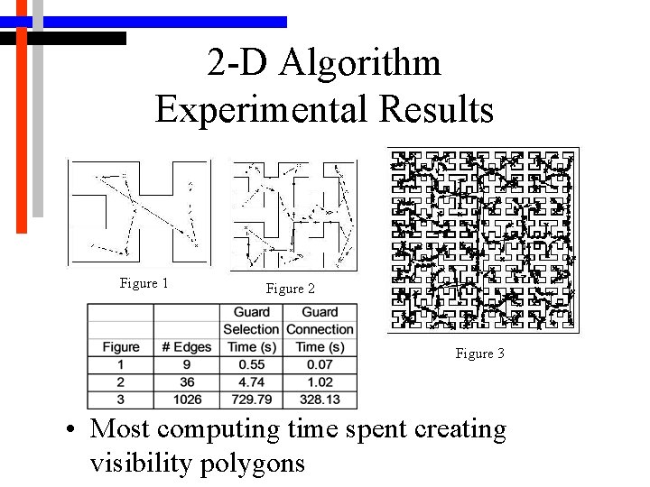
2 -D Algorithm Experimental Results Figure 1 Figure 2 Figure 3 • Most computing time spent creating visibility polygons

3 -D Algorithm • Necessary for real workspaces • Algorithm is very similar • Difficulty – computing visibility polyhedrons in 3 -D instead of visibility polygons in 2 -D

3 -D Algorithm Selecting the Guards • Visual constraints remain simple • Two steps will require visibility volumes – Determining a sampling region – Determining what surfaces a sampled point can see • However, explicitly computing visibility polyhedron can be avoided

3 -D Algorithm Selecting the Guards • Determining sampling region utilizes constraint sphere and cone – Compute the intersection of these – Randomly sample this region and test if point is valid • Both of these are much easier than computing a visibility polyhedron

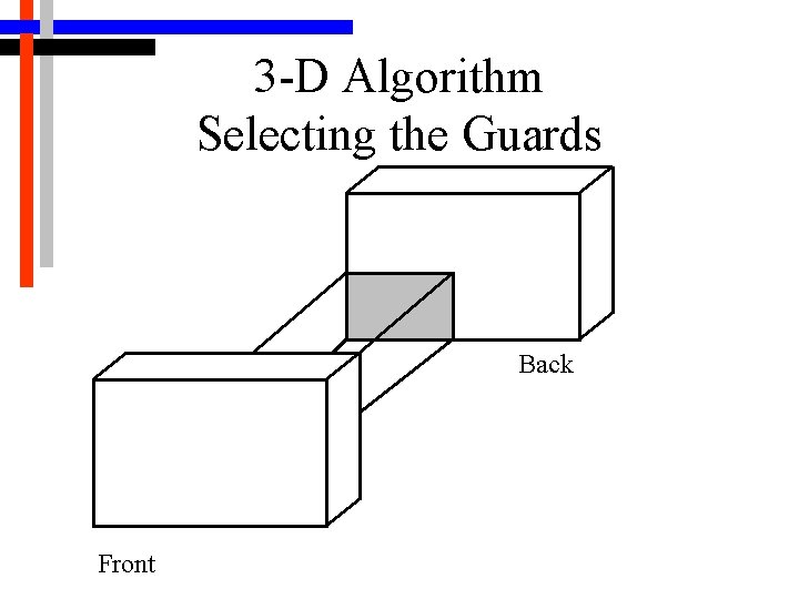
3 -D Algorithm Selecting the Guards • Once points are sampled, need to: – Determine what surfaces can be seen by them – Subtract already guarded surfaces • Use a front to back checking method, clipping each additional surface with the previous ones

3 -D Algorithm Selecting the Guards Back Front

3 -D Algorithm Selecting the Guards • Complications – Need a way of defining order – Resolving circular problems – Selecting adequate data structure • Binary Space Partitioning Tree for defining front to back order

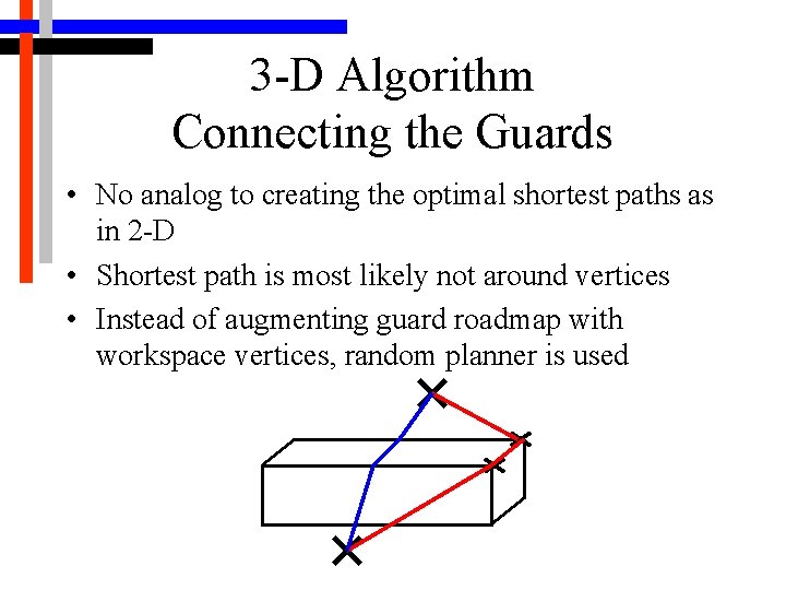
3 -D Algorithm Connecting the Guards • No analog to creating the optimal shortest paths as in 2 -D • Shortest path is most likely not around vertices • Instead of augmenting guard roadmap with workspace vertices, random planner is used

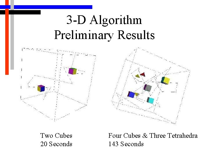
3 -D Algorithm Preliminary Results Two Cubes 20 Seconds Four Cubes & Three Tetrahedra 143 Seconds

Future Work • Considering dynamics in “path goodness” criteria • Visiting areas rather than points • Considering non-omnidirectional cameras