Randomized Composable Coresets for Submodular Maximization Morteza Zadimoghaddam

Randomized Composable Core-sets for Submodular Maximization Morteza Zadimoghaddam and Vahab Mirrokni Google Research New York

Outline • Core-sets and their Applications • Why submodular functions? • A simple algorithm for monotone and nonmonotone submodular functions. • Improving approximation factor for monotone submodular functions.

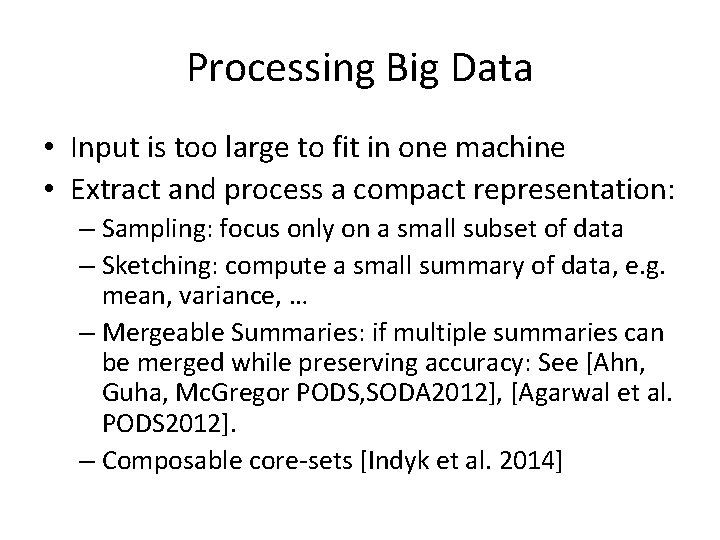
Processing Big Data • Input is too large to fit in one machine • Extract and process a compact representation: – Sampling: focus only on a small subset of data – Sketching: compute a small summary of data, e. g. mean, variance, … – Mergeable Summaries: if multiple summaries can be merged while preserving accuracy: See [Ahn, Guha, Mc. Gregor PODS, SODA 2012], [Agarwal et al. PODS 2012]. – Composable core-sets [Indyk et al. 2014]

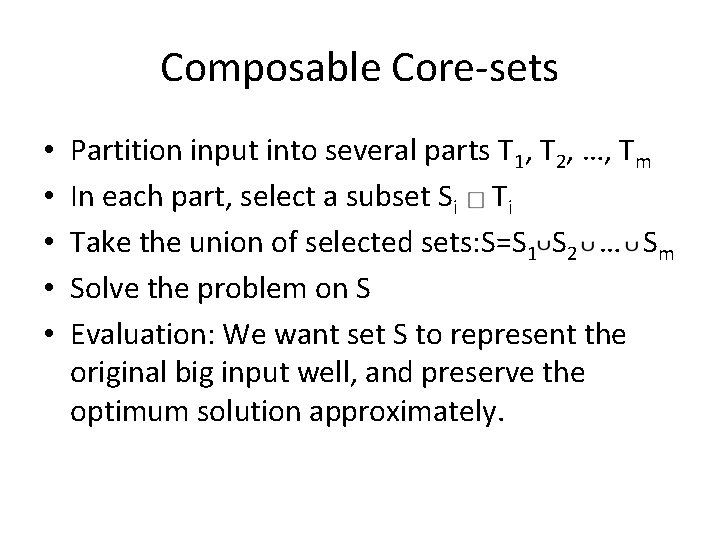
Composable Core-sets • • • Partition input into several parts T 1, T 2, …, Tm In each part, select a subset Si Ti Take the union of selected sets: S=S 1 S 2 … Sm Solve the problem on S Evaluation: We want set S to represent the original big input well, and preserve the optimum solution approximately.

Core-sets Applications • Diversity and Coverage Maximization; Indyk, Mahabadi, Mahdian, Mirrokni [PODS 2014] • k-means and k-median; Balcan et al. NIPS 2013 • Distributed Balanced Clustering; Bateni et al. NIPS 2014

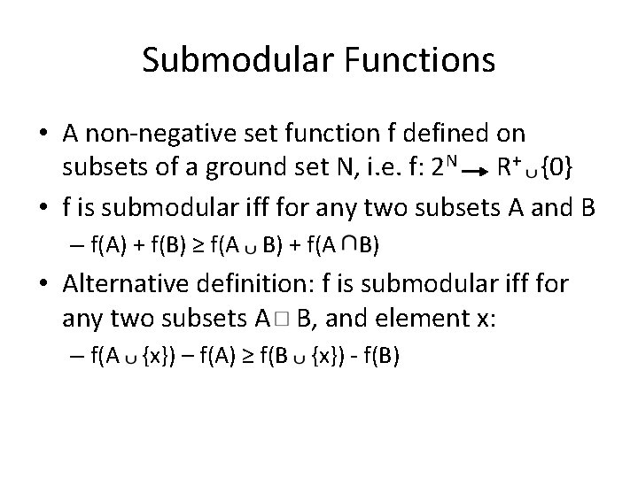
Submodular Functions • A non-negative set function f defined on subsets of a ground set N, i. e. f: 2 N R+ {0} • f is submodular iff for any two subsets A and B – f(A) + f(B) ≥ f(A B) + f(A B) • Alternative definition: f is submodular iff for any two subsets A B, and element x: – f(A {x}) – f(A) ≥ f(B {x}) - f(B)

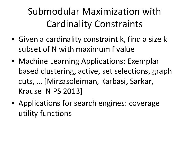
Submodular Maximization with Cardinality Constraints • Given a cardinality constraint k, find a size k subset of N with maximum f value • Machine Learning Applications: Exemplar based clustering, active, set selections, graph cuts, … [Mirzasoleiman, Karbasi, Sarkar, Krause NIPS 2013] • Applications for search engines: coverage utility functions

Submodular Maximization via Map. Reduce • Fast Greedy Algorithms in Map. Reduce and Streaming; Kumar et al. [SPAA 2013] • They get 1/2 approximation factor with super constant number of rounds

Searched Keywords with Multiple Meanings

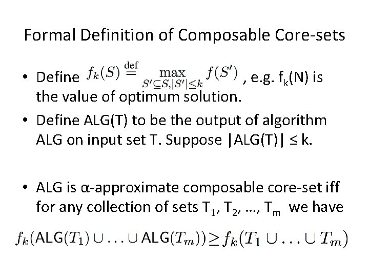
Formal Definition of Composable Core-sets • Define , e. g. fk(N) is the value of optimum solution. • Define ALG(T) to be the output of algorithm ALG on input set T. Suppose |ALG(T)| ≤ k. • ALG is α-approximate composable core-set iff for any collection of sets T 1, T 2, …, Tm we have

Applications of composable core-sets • Distributed Approximation: – Distribute input between m machines, – ALG selects set Si = ALG(Ti) in machine 1 ≤ i ≤ m, – Gather the union of selected items, S 1 S 2 … Sm , on a single machine, and select k elements. • Streaming Models: Partition the sequence of elements, and simulate the above procedure. • A class of nearest neighbor search problems

Bad News! • Theorem[Indyk et al. 2013] There exists no better than approximate composable core-set for submodular maximization

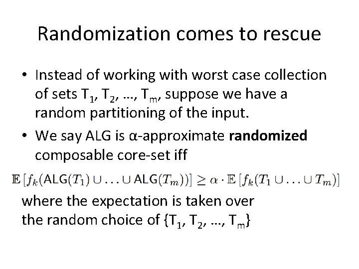
Randomization comes to rescue • Instead of working with worst case collection of sets T 1, T 2, …, Tm, suppose we have a random partitioning of the input. • We say ALG is α-approximate randomized composable core-set iff where the expectation is taken over the random choice of {T 1, T 2, …, Tm}

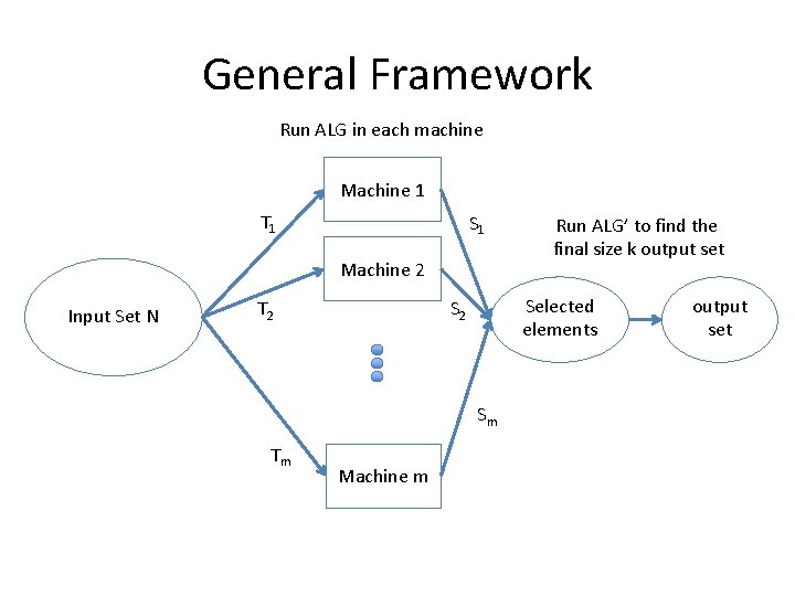
General Framework Run ALG in each machine Machine 1 T 1 S 1 Machine 2 Input Set N Selected elements S 2 T 2 Sm Tm Machine m Run ALG’ to find the final size k output set

Good news! • Theorem [Mirrokni, Z]: There exists a class of O(1)-approximate randomized composable core-sets for monotone and non-monotone submodular maximization. • In particular, algorithm Greedy is 1/3 approximate randomized core-set for monotone f, and (1/3 -1/3 m)-approximate for non-monotone f.

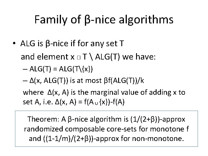
Family of β-nice algorithms • ALG is β-nice if for any set T and element x T ALG(T) we have: – ALG(T) = ALG(T{x}) – Δ(x, ALG(T)) is at most βf(ALG(T))/k where Δ(x, A) is the marginal value of adding x to set A, i. e. Δ(x, A) = f(A {x})-f(A) Theorem: A β-nice algorithm is (1/(2+β))-approx randomized composable core-sets for monotone f and ((1 -1/m)/(2+β))-approx for non-monotone.

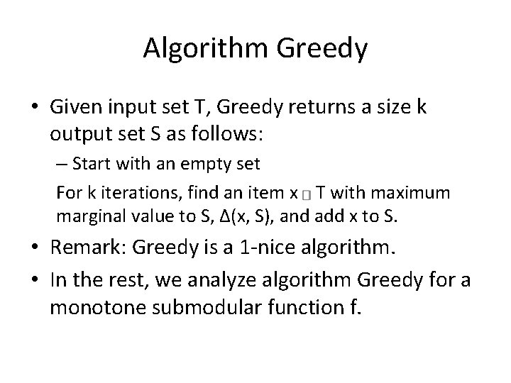
Algorithm Greedy • Given input set T, Greedy returns a size k output set S as follows: – Start with an empty set For k iterations, find an item x T with maximum marginal value to S, Δ(x, S), and add x to S. • Remark: Greedy is a 1 -nice algorithm. • In the rest, we analyze algorithm Greedy for a monotone submodular function f.

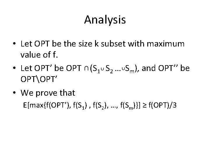
Analysis • Let OPT be the size k subset with maximum value of f. • Let OPT’ be OPT (S 1 S 2 … Sm), and OPT’’ be OPTOPT’ • We prove that E[max{f(OPT’), f(S 1) , f(S 2), …, f(Sm)}] ≥ f(OPT)/3

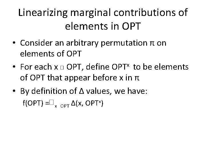
Linearizing marginal contributions of elements in OPT • Consider an arbitrary permutation π on elements of OPT • For each x OPT, define OPTx to be elements of OPT that appear before x in π • By definition of Δ values, we have: f(OPT) = x x) Δ(x, OPT

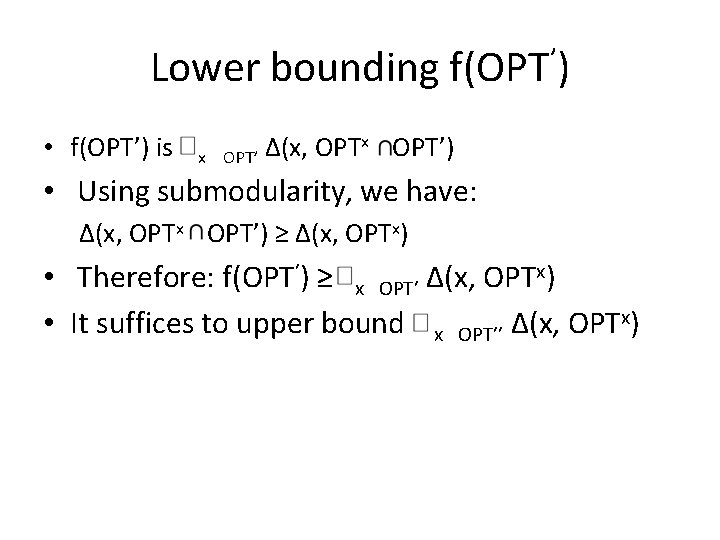
Lower bounding f(OPT’) • f(OPT’) is x x OPT’) Δ(x, OPT’ • Using submodularity, we have: Δ(x, OPTx OPT’) ≥ Δ(x, OPTx) • Therefore: f(OPT’) ≥ x OPT’ Δ(x, OPTx) • It suffices to upper bound x OPT’’ Δ(x, OPTx)

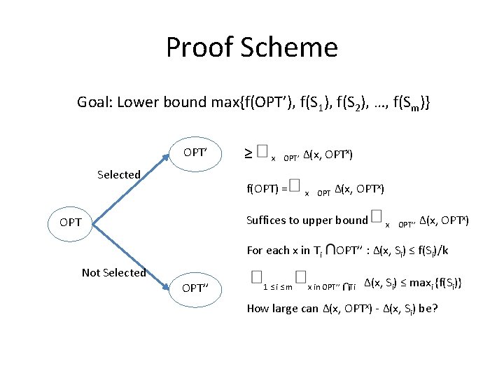
Proof Scheme Goal: Lower bound max{f(OPT’), f(S 1), f(S 2), …, f(Sm)} OPT’ Selected ≥ x OPT’ f(OPT) = Δ(x, OPTx) x OPT Δ(x, OPTx) Suffices to upper bound OPT For each x in Ti Not Selected OPT’’ 1≤i≤m x OPT’’ Δ(x, OPTx) OPT’’ : Δ(x, Si) ≤ f(Si)/k x in OPT’’ Ti Δ(x, Si) ≤ maxi {f(Si)} How large can Δ(x, OPTx) - Δ(x, Si) be?

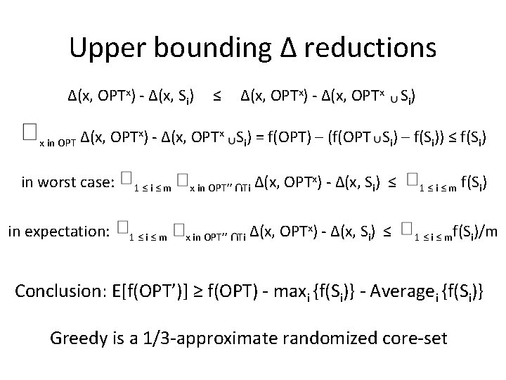
Upper bounding Δ reductions Δ(x, OPTx) - Δ(x, Si) x in OPT ≤ Δ(x, OPTx) - Δ(x, OPTx Si) = f(OPT) – (f(OPT Si) – f(Si)) ≤ f(Si) in worst case: in expectation: 1≤i≤m x in OPT’’ x) - Δ(x, S ) ≤ Δ(x, OPT Ti i x in OPT’’ Ti Δ(x, OPTx) - Δ(x, Si) ≤ 1≤i≤m f(Si) 1 ≤ i ≤ mf(Si)/m Conclusion: E[f(OPT’)] ≥ f(OPT) - maxi {f(Si)} - Averagei {f(Si)} Greedy is a 1/3 -approximate randomized core-set

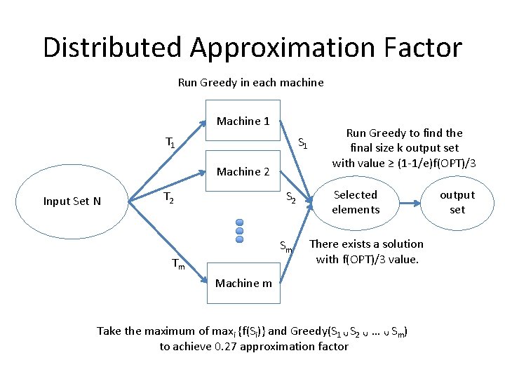
Distributed Approximation Factor Run Greedy in each machine Machine 1 T 1 S 1 Machine 2 Input Set N S 2 T 2 Sm Tm Run Greedy to find the final size k output set with value ≥ (1 -1/e)f(OPT)/3 Selected elements There exists a solution with f(OPT)/3 value. Machine m Take the maximum of maxi {f(Si)} and Greedy(S 1 S 2 … Sm) to achieve 0. 27 approximation factor output set

Improving Approximation Factors for Monotone Submodular Functions • Hardness Result [Mirrokni, Z]: With output sizes (|Si|) ≤ k, Greedy, and locally optimum algorithms are not better than ½ approximate randomized core-sets. • Can we increase the output sizes and get better results?

-approximate Randomized Core-set • Positive Result [Mirrokni, Z]: If we increase the output sizes to be 4 k, Greedy will be (2 -√ 2)o(1) ≥ 0. 585 -approximate randomized core-set for a monotone submodular function. • Remark: In this result, we send each item to C random machines instead of one. As a result, the approximation factors are reduced by a O(ln(C)/C) term.

0. 545 Distributed Approximation Factor • If we run Greedy again at the second stage, the distributed approximation factor will be 0. 585(1 -1/e) < 0. 37. • Positive Distributed Result [Mirrokni, Z]: We propose a new algorithm Pseudo. Greedy for the with distributed approximation factor 0. 545. We still use Greedy in the first stage to return 4 k elements in each machine.

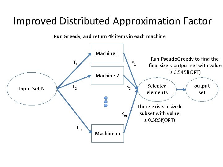
Improved Distributed Approximation Factor Run Greedy, and return 4 k items in each machine Machine 1 T 1 S 1 Machine 2 Input Set N S 2 T 2 Sm Tm Machine m Run Pseudo. Greedy to find the final size k output set with value ≥ 0. 545 f(OPT) Selected elements There exists a size k subset with value ≥ 0. 585 f(OPT) output set

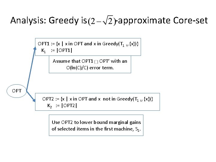
Analysis: Greedy is -approximate Core-set OPT 1 : = {x | x in OPT and x in Greedy(T 1 {x})} K 1 : = |OPT 1| Assume that OPT 1 OPT’ with an O(ln(C)/C) error term. OPT 2 : = {x | x in OPT and x not in Greedy(T 1 {x})} K 2 : = |OPT 2| Use OPT 2 to lower bound marginal gains of selected items in the first machine, S 1.

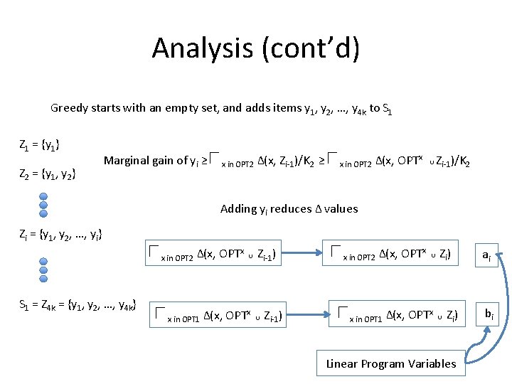
Analysis (cont’d) Greedy starts with an empty set, and adds items y 1, y 2, …, y 4 k to S 1 Z 1 = {y 1} Z 2 = {y 1, y 2} Marginal gain of yi ≥ x in OPT 2 Δ(x, Zi-1)/K 2 ≥ x in OPT 2 Δ(x, OPTx Zi-1)/K 2 Δ(x, OPTx Zi ) Adding yi reduces Δ values Zi = {y 1, y 2, …, yi} x in OPT 2 Δ(x, OPTx S 1 = Z 4 k = {y 1, y 2, …, y 4 k} x in OPT 1 Δ(x, OPTx Zi-1) x in OPT 2 x in OPT 1 Δ(x, OPTx Zi ) Linear Program Variables ai bi

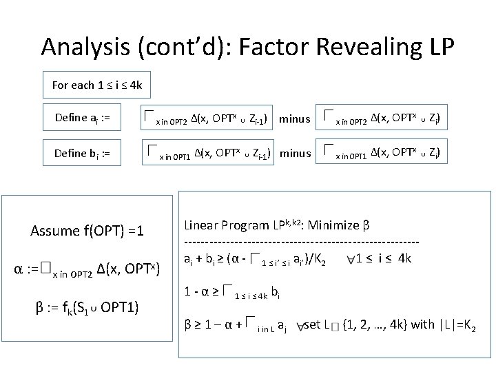
Analysis (cont’d): Factor Revealing LP For each 1 ≤ i ≤ 4 k Define ai : = Define bi : = x in OPT 2 Δ(x, OPTx) β : = fk(S 1 OPT 1) Zi-1) minus x in OPT 2 Δ(x, OPTx Zi ) Δ(x, OPTx Zi-1) minus x in OPT 1 Δ(x, OPTx Zi ) x in OPT 1 Assume f(OPT) =1 α : = Δ(x, OPTx Linear Program LPk, k 2: Minimize β ----------------------------ai + bi ≥ (α - 1 ≤ i’ ≤ i ai’)/K 2 1 ≤ i ≤ 4 k 1 -α≥ 1 ≤ i ≤ 4 k β≥ 1–α+ bi i in L aj set L {1, 2, …, 4 k} with |L|=K 2

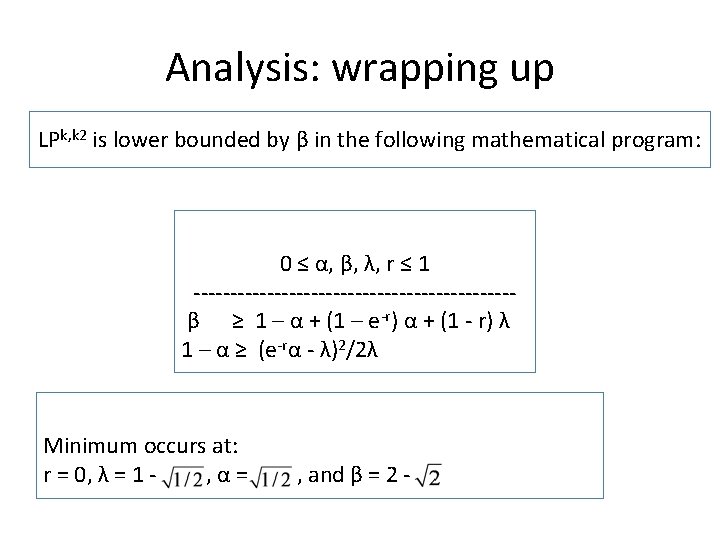
Analysis: wrapping up LPk, k 2 is lower bounded by β in the following mathematical program: 0 ≤ α, β, λ, r ≤ 1 ----------------------β ≥ 1 – α + (1 – e-r) α + (1 - r) λ 1 – α ≥ (e-rα - λ)2/2λ Minimum occurs at: r = 0, λ = 1 , α= , and β = 2 -

Improved Distributed Approximation Factor Run Greedy, and return 4 k items in each machine Machine 1 T 1 S 1 Machine 2 Input Set N S 2 T 2 Sm Tm Machine m Run Pseudo. Greedy to find the final size k output set with value ≥ 0. 545 f(OPT) Selected elements There exists a size k subset with value ≥ 0. 585 f(OPT) output set

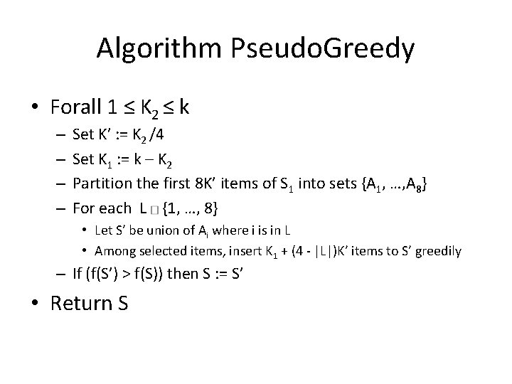
Algorithm Pseudo. Greedy • Forall 1 ≤ K 2 ≤ k – – Set K’ : = K 2 /4 Set K 1 : = k – K 2 Partition the first 8 K’ items of S 1 into sets {A 1, …, A 8} For each L {1, …, 8} • Let S’ be union of Ai where i is in L • Among selected items, insert K 1 + (4 - |L|)K’ items to S’ greedily – If (f(S’) > f(S)) then S : = S’ • Return S

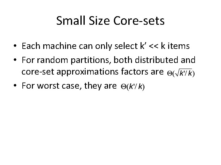
Small Size Core-sets • Each machine can only select k’ << k items • For random partitions, both distributed and core-set approximations factors are • For worst case, they are

Thank you! Questions?