Random Walks on Graphs An Overview Purnamrita Sarkar

Random Walks on Graphs: An Overview Purnamrita Sarkar 1

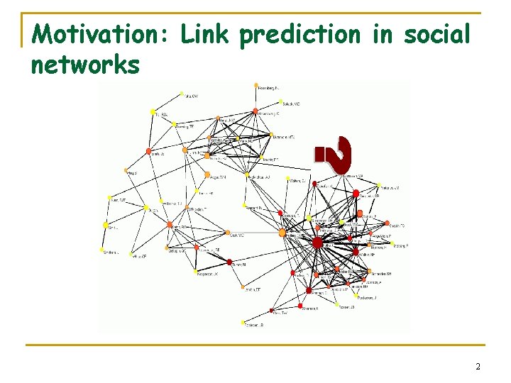
Motivation: Link prediction in social networks 2

Motivation: Basis for recommendation 3

Motivation: Personalized search 4

Why graphs? n The underlying data is naturally a graph q q q Papers linked by citation Authors linked by co-authorship Bipartite graph of customers and products Web-graph Friendship networks: who knows whom 5

What are we looking for n Rank nodes for a particular query q q q Top k matches for “Random Walks” from Citeseer Who are the most likely co-authors of “Manuel Blum”. Top k book recommendations for Purna from Amazon Top k websites matching “Sound of Music” Top k friend recommendations for Purna when she joins “Facebook” 6

Talk Outline n Basic definitions q q n Random walks Stationary distributions Properties q q Perron frobenius theorem Electrical networks, hitting and commute times n n Euclidean Embedding Applications q Pagerank n n q q Power iteration Convergencce Personalized pagerank Rank stability 7

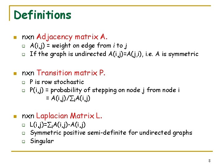
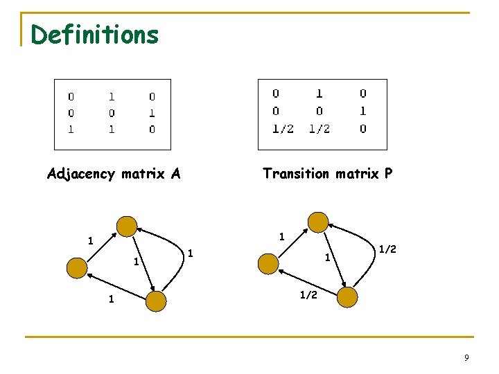
Definitions n nxn Adjacency matrix A. q q n nxn Transition matrix P. q q n A(i, j) = weight on edge from i to j If the graph is undirected A(i, j)=A(j, i), i. e. A is symmetric P is row stochastic P(i, j) = probability of stepping on node j from node i = A(i, j)/∑i. A(i, j) nxn Laplacian Matrix L. q q q L(i, j)=∑i. A(i, j)-A(i, j) Symmetric positive semi-definite for undirected graphs Singular 8

Definitions Adjacency matrix A Transition matrix P 1 1 1 1/2 9

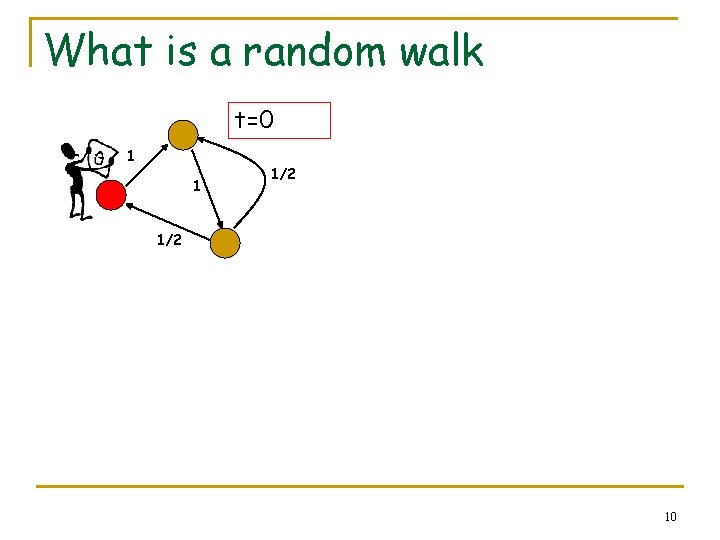
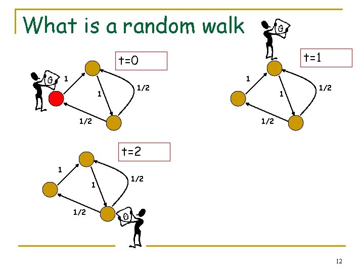
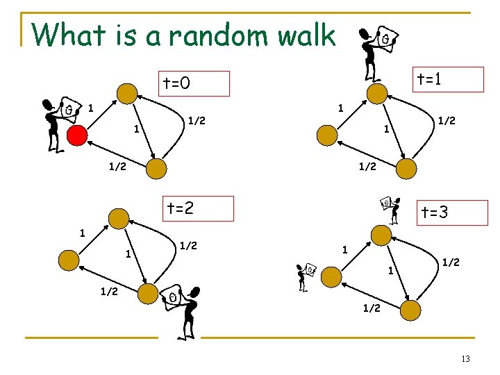
What is a random walk t=0 1 1 1/2 10

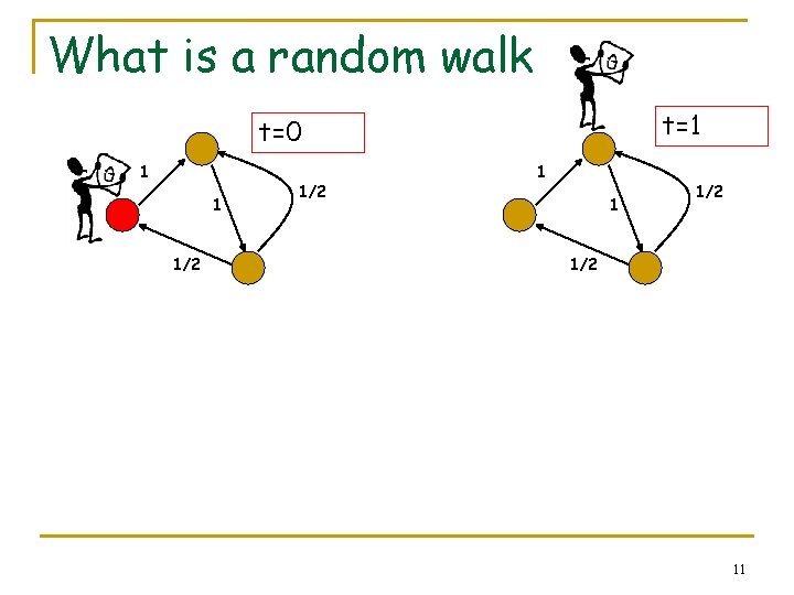
What is a random walk t=1 t=0 1 1 1/2 1/2 11

What is a random walk t=1 t=0 1 1 1/2 1/2 t=2 1 1 1/2 12

What is a random walk t=1 t=0 1 1 1/2 1/2 t=2 1 1 1/2 t=3 1 1 1/2 1/2 13

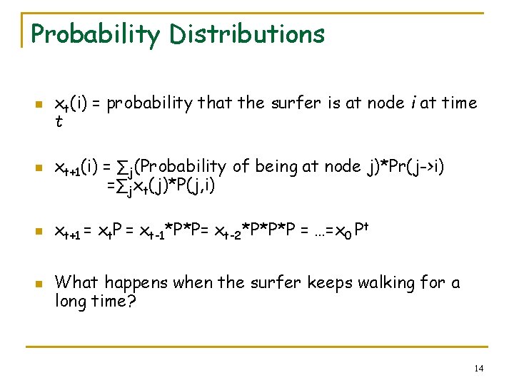
Probability Distributions n n xt(i) = probability that the surfer is at node i at time t xt+1(i) = ∑j(Probability of being at node j)*Pr(j->i) =∑jxt(j)*P(j, i) xt+1 = xt. P = xt-1*P*P= xt-2*P*P*P = …=x 0 Pt What happens when the surfer keeps walking for a long time? 14

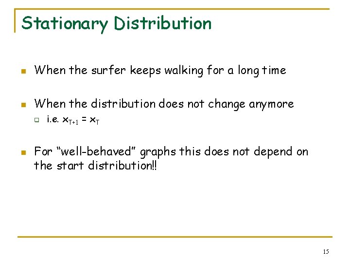
Stationary Distribution n When the surfer keeps walking for a long time n When the distribution does not change anymore q n i. e. x. T+1 = x. T For “well-behaved” graphs this does not depend on the start distribution!! 15

What is a stationary distribution? Intuitively and Mathematically 16

What is a stationary distribution? Intuitively and Mathematically n The stationary distribution at a node is related to the amount of time a random walker spends visiting that node. 17

What is a stationary distribution? Intuitively and Mathematically n n The stationary distribution at a node is related to the amount of time a random walker spends visiting that node. Remember that we can write the probability distribution at a node as q xt+1 = xt. P 18

What is a stationary distribution? Intuitively and Mathematically n n n The stationary distribution at a node is related to the amount of time a random walker spends visiting that node. Remember that we can write the probability distribution at a node as q xt+1 = xt. P For the stationary distribution v 0 we have q v 0 = v 0 P 19

What is a stationary distribution? Intuitively and Mathematically n n The stationary distribution at a node is related to the amount of time a random walker spends visiting that node. Remember that we can write the probability distribution at a node as q xt+1 = xt. P For the stationary distribution v 0 we have q v 0 = v 0 P Whoa! that’s just the left eigenvector of the transition matrix ! 20

Talk Outline n Basic definitions q q n Random walks Stationary distributions Properties q q Perron frobenius theorem Electrical networks, hitting and commute times n n Euclidean Embedding Applications q Pagerank n n q q Power iteration Convergencce Personalized pagerank Rank stability 21

Interesting questions n Does a stationary distribution always exist? Is it unique? q n What is “well-behaved”? q n Yes, if the graph is “well-behaved”. We shall talk about this soon. How fast will the random surfer approach this stationary distribution? q Mixing Time! 22

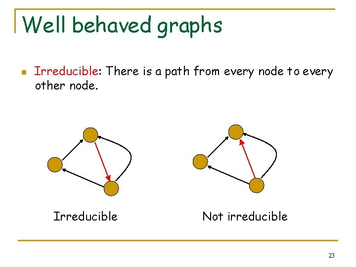
Well behaved graphs n Irreducible: There is a path from every node to every other node. Irreducible Not irreducible 23

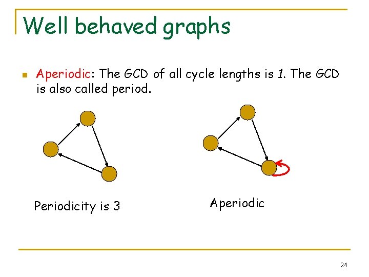
Well behaved graphs n Aperiodic: The GCD of all cycle lengths is 1. The GCD is also called period. Periodicity is 3 Aperiodic 24

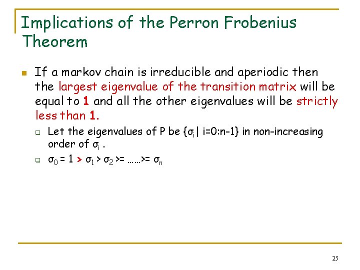
Implications of the Perron Frobenius Theorem n If a markov chain is irreducible and aperiodic then the largest eigenvalue of the transition matrix will be equal to 1 and all the other eigenvalues will be strictly less than 1. q q Let the eigenvalues of P be {σi| i=0: n-1} in non-increasing order of σi. σ0 = 1 > σ2 >= ……>= σn 25

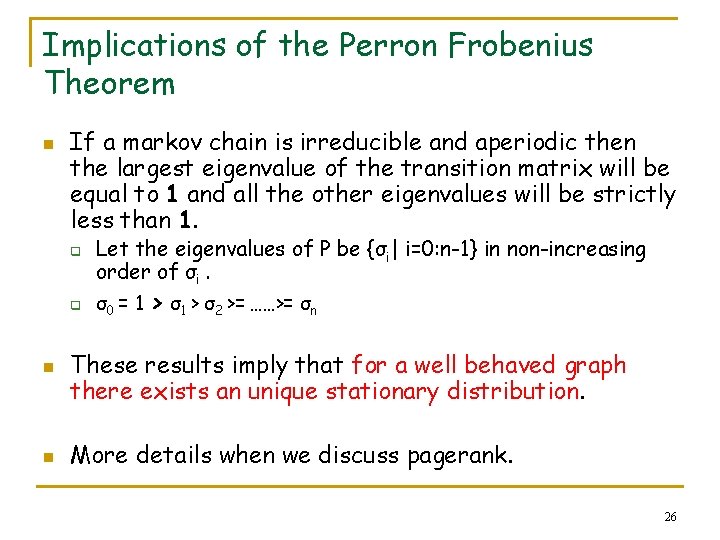
Implications of the Perron Frobenius Theorem n If a markov chain is irreducible and aperiodic then the largest eigenvalue of the transition matrix will be equal to 1 and all the other eigenvalues will be strictly less than 1. q q n n Let the eigenvalues of P be {σi| i=0: n-1} in non-increasing order of σi. σ0 = 1 > σ2 >= ……>= σn These results imply that for a well behaved graph there exists an unique stationary distribution. More details when we discuss pagerank. 26

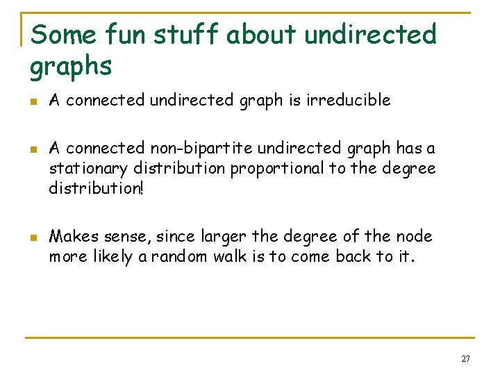
Some fun stuff about undirected graphs n n n A connected undirected graph is irreducible A connected non-bipartite undirected graph has a stationary distribution proportional to the degree distribution! Makes sense, since larger the degree of the node more likely a random walk is to come back to it. 27

Talk Outline n Basic definitions q q n Random walks Stationary distributions Properties q q Perron frobenius theorem Electrical networks, hitting and commute times n n Euclidean Embedding Applications q Pagerank n n q q Power iteration Convergencce Personalized pagerank Rank stability 28

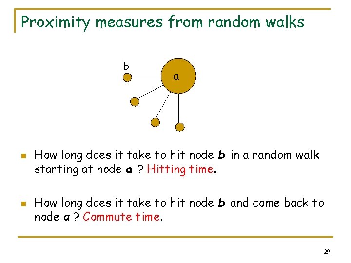
Proximity measures from random walks b n n a How long does it take to hit node b in a random walk starting at node a ? Hitting time. How long does it take to hit node b and come back to node a ? Commute time. 29

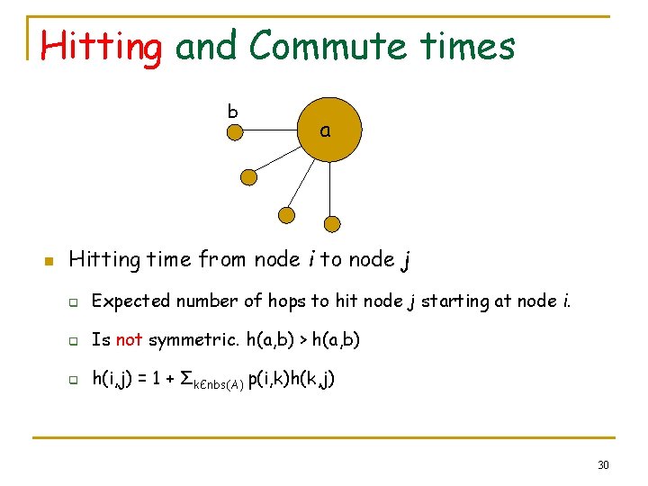
Hitting and Commute times b n a Hitting time from node i to node j q Expected number of hops to hit node j starting at node i. q Is not symmetric. h(a, b) > h(a, b) q h(i, j) = 1 + ΣkЄnbs(A) p(i, k)h(k, j) 30

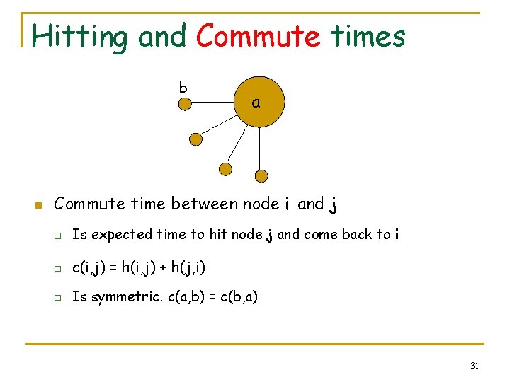
Hitting and Commute times b n a Commute time between node i and j q Is expected time to hit node j and come back to i q c(i, j) = h(i, j) + h(j, i) q Is symmetric. c(a, b) = c(b, a) 31

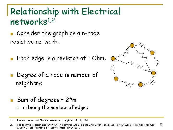
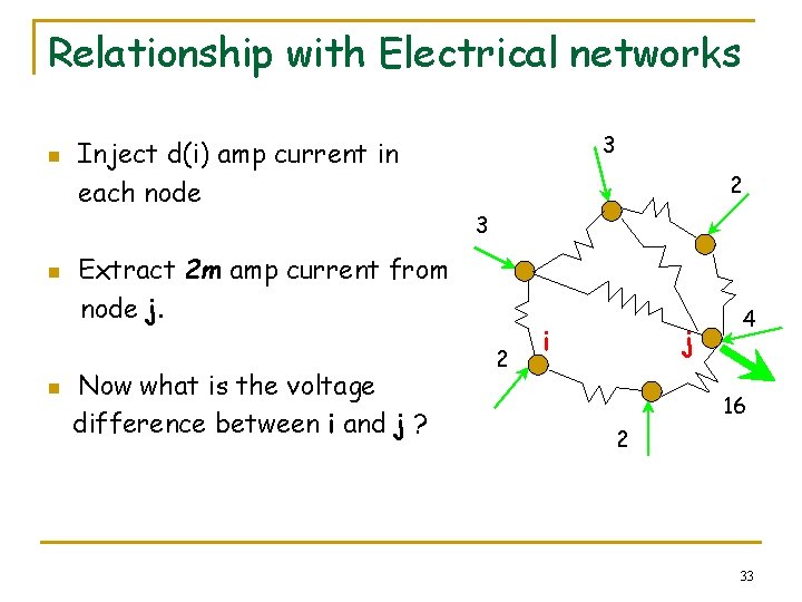
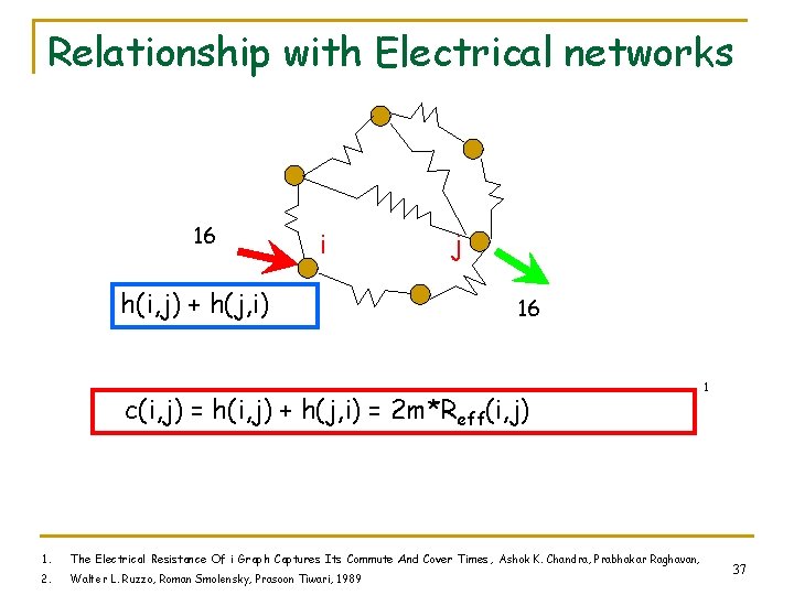
Relationship with Electrical networks 1, 2 Consider the graph as a n-node resistive network. n n Each edge is a resistor of 1 Ohm. Degree of a node is number of neighbors Sum of degrees = 2*m q m being the number of edges 1. Random Walks and Electric Networks , Doyle and Snell, 1984 2. The Electrical Resistance Of A Graph Captures Its Commute And Cover Times, Ashok K. Chandra, Prabhakar Raghavan, Walter L. Ruzzo, Roman Smolensky, Prasoon Tiwari, 1989 32

Relationship with Electrical networks n n n Inject d(i) amp current in each node 3 2 3 Extract 2 m amp current from node j. Now what is the voltage difference between i and j ? 2 i j 4 16 2 33

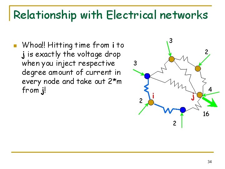
Relationship with Electrical networks n Whoa!! Hitting time from i to j is exactly the voltage drop when you inject respective degree amount of current in every node and take out 2*m from j! 3 2 i j 4 16 2 34

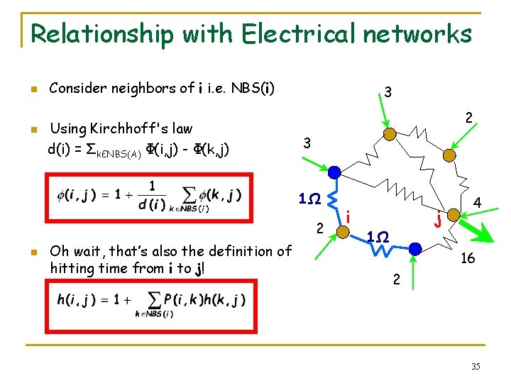
Relationship with Electrical networks n n Consider neighbors of i i. e. NBS(i) Using Kirchhoff's law d(i) = ΣkЄNBS(A) Φ(i, j) - Φ(k, j) 3 2 3 1Ω 2 n Oh wait, that’s also the definition of hitting time from i to j! i j 1Ω 4 16 2 35

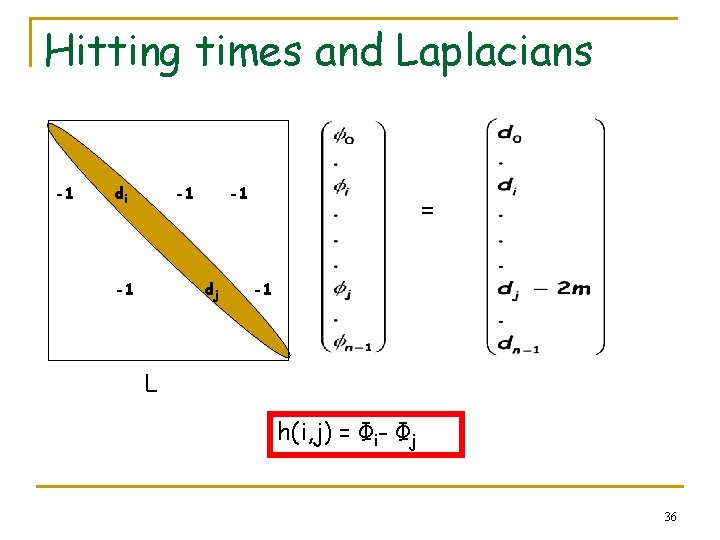
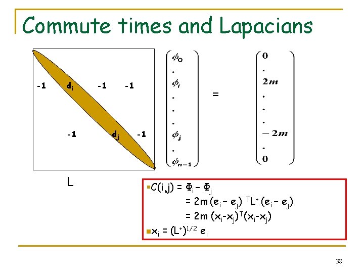
Hitting times and Laplacians -1 di -1 -1 -1 dj = -1 L h(i, j) = Φi- Φj 36

Relationship with Electrical networks 16 i h(i, j) + h(j, i) j 16 c(i, j) = h(i, j) + h(j, i) = 2 m*Reff(i, j) 1. The Electrical Resistance Of i Graph Captures Its Commute And Cover Times, Ashok K. Chandra, Prabhakar Raghavan, 2. Walter L. Ruzzo, Roman Smolensky, Prasoon Tiwari, 1989 1 37

Commute times and Lapacians -1 di -1 L -1 -1 dj = -1 §C(i, j) = Φi – Φj = 2 m (ei – ej) TL+ (ei – ej) = 2 m (xi-xj)T(xi-xj) nxi = (L+)1/2 ei 38

Commute times and Laplacians n n Why is this interesting ? Because, this gives a very intuitive definition of embedding the points in some Euclidian space, s. t. the commute times is the squared Euclidian distances in the transformed space. 1 1. The Principal Components Analysis of a Graph, and its Relationships to Spectral Clustering. M. Saerens, et al, ECML ‘ 04 39

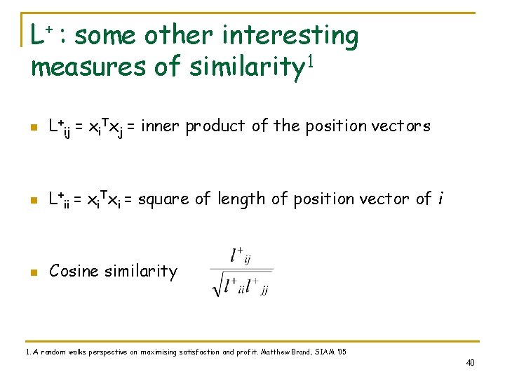
L+ : some other interesting measures of similarity 1 n L+ij = xi. Txj = inner product of the position vectors n L+ii = xi. Txi = square of length of position vector of i n Cosine similarity 1. A random walks perspective on maximising satisfaction and profit. Matthew Brand, SIAM ‘ 05 40

Talk Outline n Basic definitions q q n Random walks Stationary distributions Properties q q Perron frobenius theorem Electrical networks, hitting and commute times n n Euclidean Embedding Applications q q Recommender Networks Pagerank n n q q Power iteration Convergencce Personalized pagerank Rank stability 41

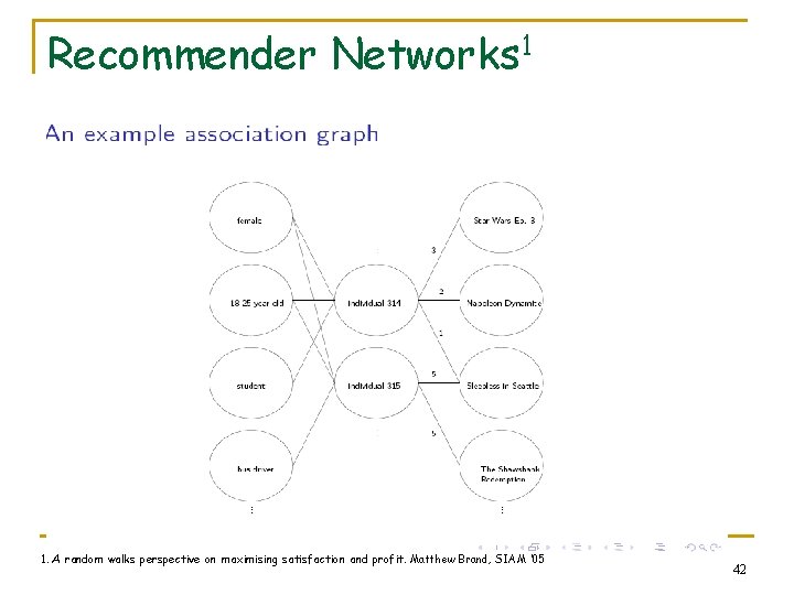
Recommender Networks 1 1. A random walks perspective on maximising satisfaction and profit. Matthew Brand, SIAM ‘ 05 42

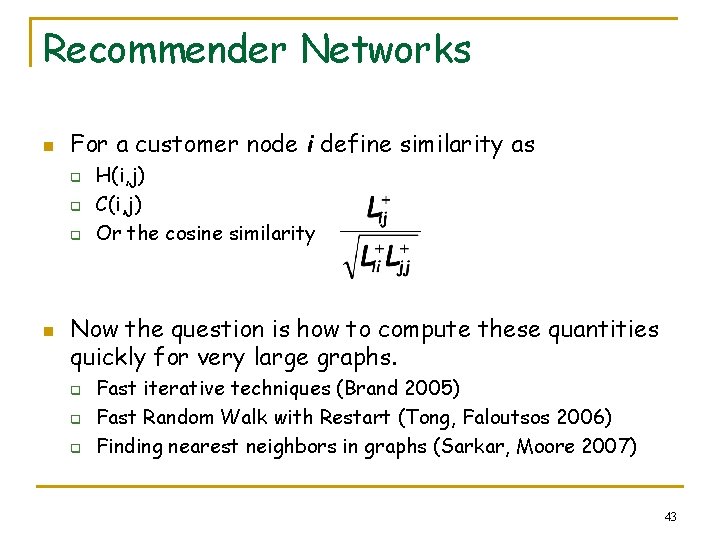
Recommender Networks n For a customer node i define similarity as q q q n H(i, j) C(i, j) Or the cosine similarity Now the question is how to compute these quantities quickly for very large graphs. q q q Fast iterative techniques (Brand 2005) Fast Random Walk with Restart (Tong, Faloutsos 2006) Finding nearest neighbors in graphs (Sarkar, Moore 2007) 43

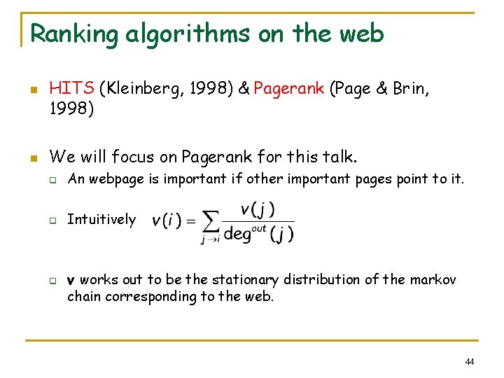
Ranking algorithms on the web n n HITS (Kleinberg, 1998) & Pagerank (Page & Brin, 1998) We will focus on Pagerank for this talk. q An webpage is important if other important pages point to it. q Intuitively q v works out to be the stationary distribution of the markov chain corresponding to the web. 44

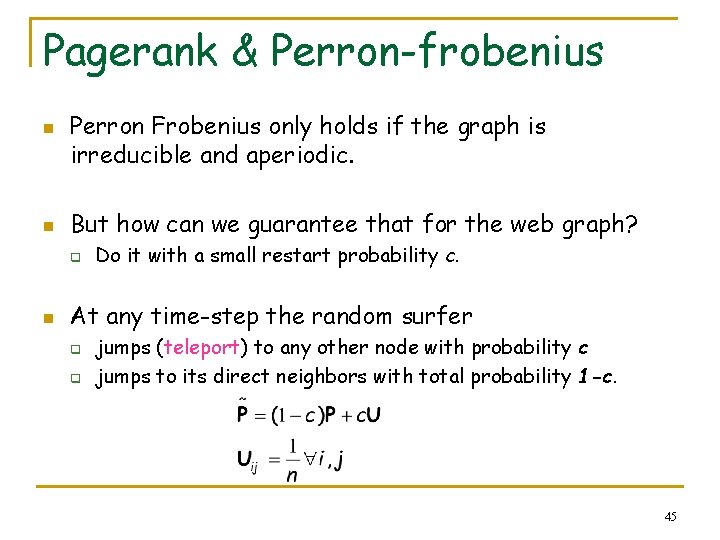
Pagerank & Perron-frobenius n n Perron Frobenius only holds if the graph is irreducible and aperiodic. But how can we guarantee that for the web graph? q n Do it with a small restart probability c. At any time-step the random surfer q q jumps (teleport) to any other node with probability c jumps to its direct neighbors with total probability 1 -c. 45

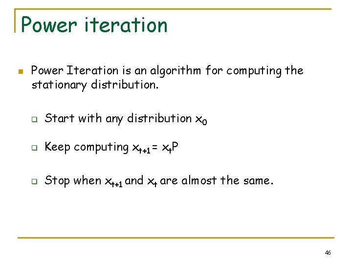
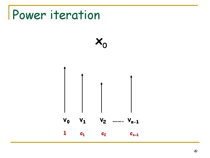
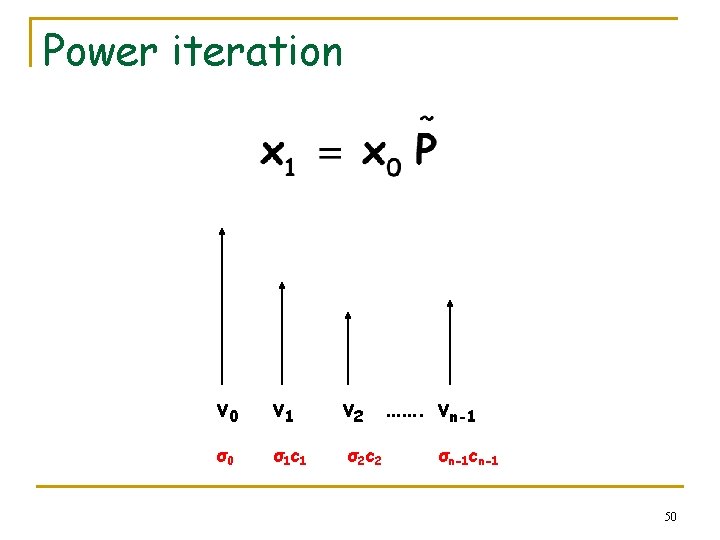
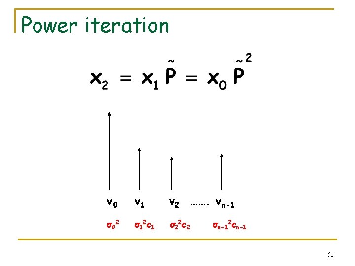
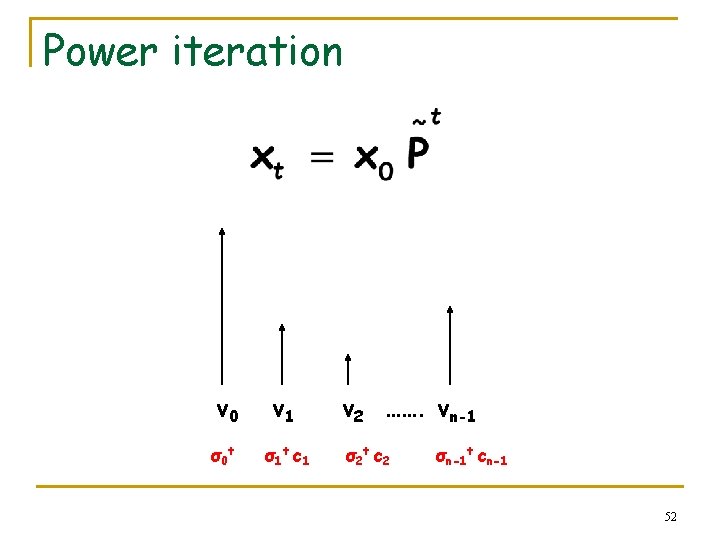
Power iteration n Power Iteration is an algorithm for computing the stationary distribution. q Start with any distribution x 0 q Keep computing xt+1 = xt. P q Stop when xt+1 and xt are almost the same. 46

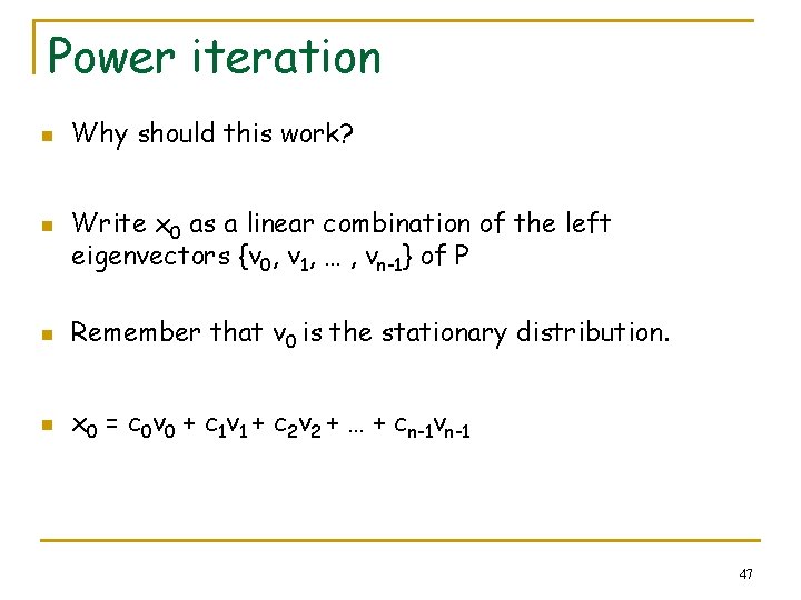
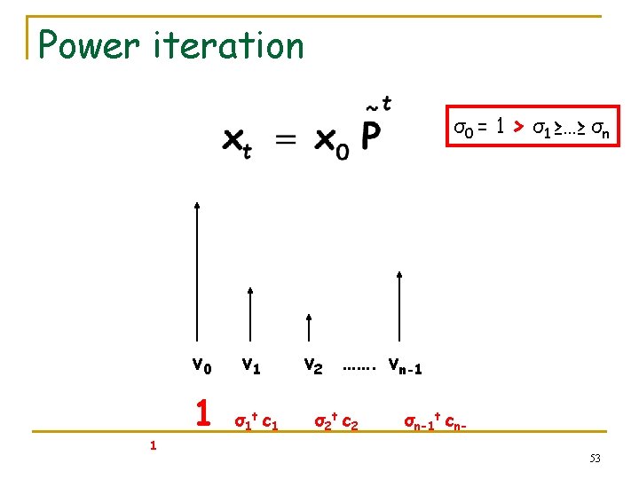
Power iteration n n Why should this work? Write x 0 as a linear combination of the left eigenvectors {v 0, v 1, … , vn-1} of P n Remember that v 0 is the stationary distribution. n x 0 = c 0 v 0 + c 1 v 1 + c 2 v 2 + … + cn-1 vn-1 47

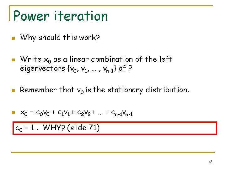
Power iteration n n Why should this work? Write x 0 as a linear combination of the left eigenvectors {v 0, v 1, … , vn-1} of P n Remember that v 0 is the stationary distribution. n x 0 = c 0 v 0 + c 1 v 1 + c 2 v 2 + … + cn-1 vn-1 c 0 = 1. WHY? (slide 71) 48

Power iteration v 0 v 1 v 2 ……. vn-1 1 c 2 cn-1 49

Power iteration v 0 v 1 σ0 σ 1 c 1 v 2 ……. vn-1 σ 2 c 2 σn-1 cn-1 50

Power iteration v 0 v 1 v 2 ……. vn-1 σ 02 σ 12 c 1 σ 22 c 2 σn-12 cn-1 51

Power iteration v 0 v 1 σ 0 t σ 1 t c 1 v 2 ……. vn-1 σ 2 t c 2 σn-1 t cn-1 52

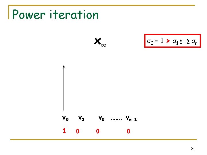
Power iteration σ0 = 1 > σ1 ≥…≥ σn v 0 1 1 v 1 σ1 t c 1 v 2 ……. vn-1 σ2 t c 2 σn-1 t cn 53

Power iteration σ0 = 1 > σ1 ≥…≥ σn v 0 1 v 1 0 v 2 ……. vn-1 0 0 54

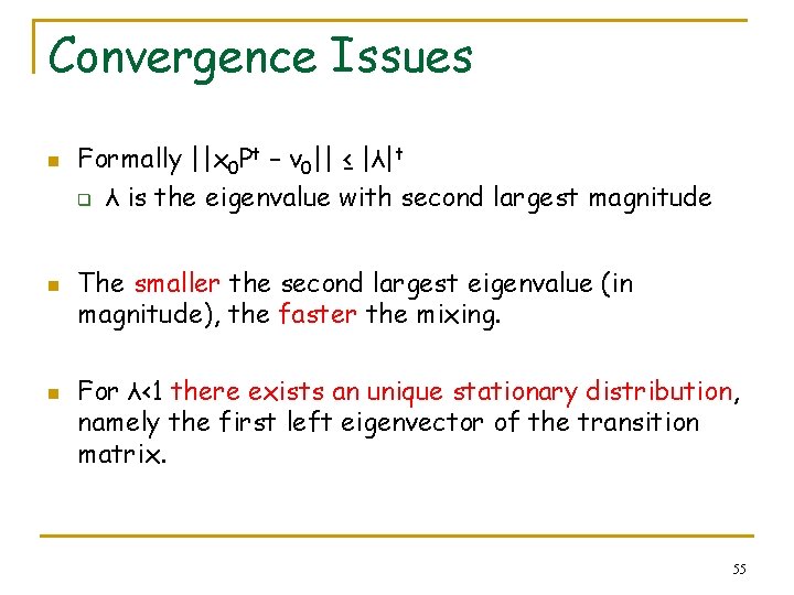
Convergence Issues n n n Formally ||x 0 Pt – v 0|| ≤ |λ|t q λ is the eigenvalue with second largest magnitude The smaller the second largest eigenvalue (in magnitude), the faster the mixing. For λ<1 there exists an unique stationary distribution, namely the first left eigenvector of the transition matrix. 55

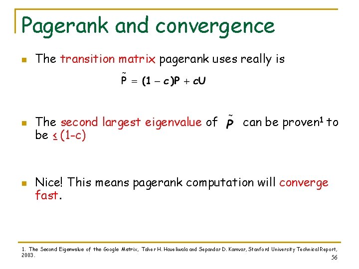
Pagerank and convergence n n n The transition matrix pagerank uses really is The second largest eigenvalue of be ≤ (1 -c) can be proven 1 to Nice! This means pagerank computation will converge fast. 1. The Second Eigenvalue of the Google Matrix, Taher H. Haveliwala and Sepandar D. Kamvar, Stanford University Technical Report, 2003. 56

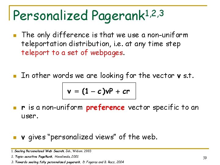
Pagerank n We are looking for the vector v s. t. n r is a distribution over web-pages. n If r is the uniform distribution we get pagerank. n What happens if r is non-uniform? 57

Pagerank n We are looking for the vector v s. t. n r is a distribution over web-pages. n If r is the uniform distribution we get pagerank. n What happens if r is non-uniform? Personalization 58

Personalized Pagerank 1, 2, 3 n n The only difference is that we use a non-uniform teleportation distribution, i. e. at any time step teleport to a set of webpages. In other words we are looking for the vector v s. t. r is a non-uniform preference vector specific to an user. v gives “personalized views” of the web. 1. Scaling Personalized Web Search, Jeh, Widom. 2003 2. Topic-sensitive Page. Rank, Haveliwala, 2001 3. Towards scaling fully personalized pagerank, D. Fogaras and B. Racz, 2004 59

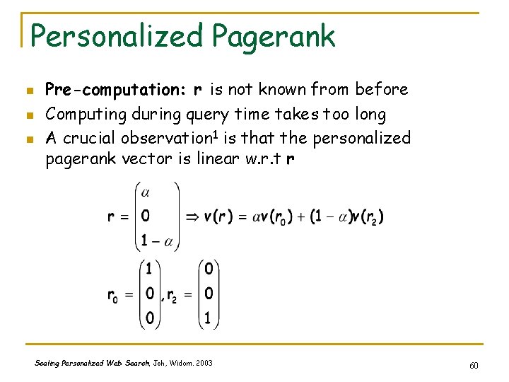
Personalized Pagerank n n n Pre-computation: r is not known from before Computing during query time takes too long A crucial observation 1 is that the personalized pagerank vector is linear w. r. t r Scaling Personalized Web Search, Jeh, Widom. 2003 60

Topic-sensitive pagerank (Haveliwala’ 01) n n n Divide the webpages into 16 broad categories For each category compute the biased personalized pagerank vector by uniformly teleporting to websites under that category. At query time the probability of the query being from any of the above classes is computed, and the final page-rank vector is computed by a linear combination of the biased pagerank vectors computed offline. 61

Personalized Pagerank: Other Approaches n n n Scaling Personalized Web Search (Jeh & Widom ’ 03) Towards scaling fully personalized pagerank: algorithms, lower bounds and experiments (Fogaras et al, 2004) Dynamic personalized pagerank in entity-relation graphs. (Soumen Chakrabarti, 2007) 62

Personalized Pagerank (Purna’s Take) n n But, whats the guarantee that the new transition matrix will still be irreducible? Check out q q n The Second Eigenvalue of the Google Matrix, Taher H. Haveliwala and Sepandar D. Kamvar, Stanford University Technical Report, 2003. Deeper Inside Page. Rank, Amy N. Langville. and Carl D. Meyer. Internet Mathematics, 2004. As long as you are adding any rank one (where the matrix is a repetition of one distinct row) matrix of form (1 Tr) to your transition matrix as shown before, q λ ≤ 1 -c 63

Talk Outline n Basic definitions q q n Random walks Stationary distributions Properties q q Perron frobenius theorem Electrical networks, hitting and commute times n n Euclidean Embedding Applications q q Recommender Networks Pagerank n n q q Power iteration Convergence Personalized pagerank Rank stability 64

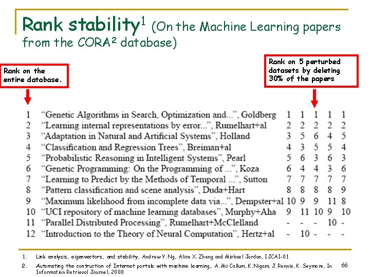
Rank stability n How does the ranking change when the link structure changes? n The web-graph is changing continuously. n How does that affect page-rank? 65

Rank stability 1 (On the Machine Learning papers from the CORA 2 database) Rank on the entire database. Rank on 5 perturbed datasets by deleting 30% of the papers 1. Link analysis, eigenvectors, and stability, Andrew Y. Ng, Alice X. Zheng and Michael Jordan, IJCAI-01 2. Automating the contruction of Internet portals with machine learning, A. Mc Callum, K. Nigam, J. Rennie, K. Seymore, In Information Retrieval Journel, 2000 66

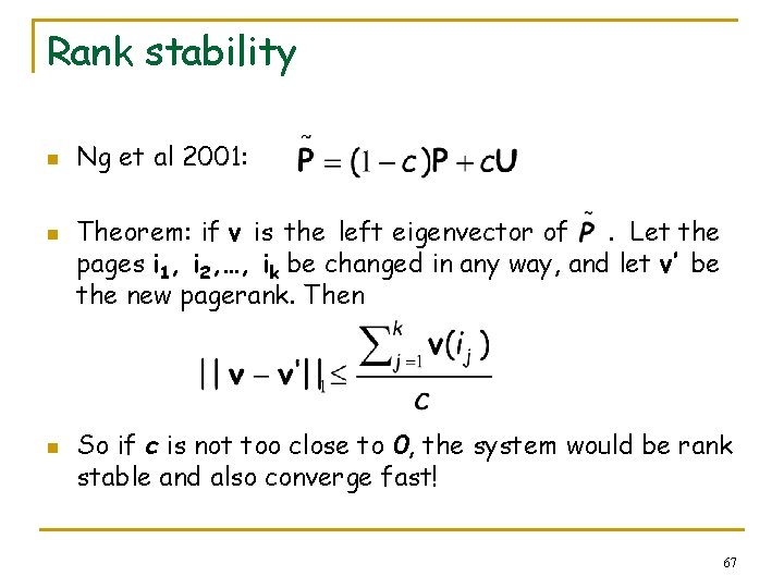
Rank stability n n n Ng et al 2001: Theorem: if v is the left eigenvector of. Let the pages i 1, i 2, …, ik be changed in any way, and let v’ be the new pagerank. Then So if c is not too close to 0, the system would be rank stable and also converge fast! 67

Conclusion n Basic definitions q q n Random walks Stationary distributions Properties q q Perron frobenius theorem Electrical networks, hitting and commute times n n Euclidean Embedding Applications q Pagerank n n q q Power iteration Convergencce Personalized pagerank Rank stability 68

Thanks! Please send email to Purna at psarkar@cs. cmu. edu with questions, suggestions, corrections 69

Acknowledgements n Andrew Moore n Gary Miller q q n Fan Chung Graham’s course on q q n n n Check out Gary’s Fall 2007 class on “Spectral Graph Theory, Scientific Computing, and Biomedical Applications” http: //www. cs. cmu. edu/afs/cs/user/glmiller/public/Scientific. Computing/F-07/index. html Random Walks on Directed and Undirected Graphs http: //www. math. ucsd. edu/~phorn/math 261/ Random Walks on Graphs: A Survey, Laszlo Lov'asz Reversible Markov Chains and Random Walks on Graphs, D Aldous, J Fill Random Walks and Electric Networks, Doyle & Snell 70

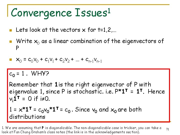
Convergence Issues 1 n n n Lets look at the vectors x for t=1, 2, … Write x 0 as a linear combination of the eigenvectors of P x 0 = c 0 v 0 + c 1 v 1 + c 2 v 2 + … + cn-1 vn-1 c 0 = 1. WHY? Remember that 1 is the right eigenvector of P with eigenvalue 1, since P is stochastic. i. e. P*1 T = 1 T. Hence vi 1 T = 0 if i≠ 0. 1 = x*1 T = c 0 v 0*1 T = c 0. Since v 0 and x 0 are both distributions 1. We are assuming that P is diagonalizable. The non-diagonalizable case is trickier, you can take a look at Fan Chung Graham’s class notes (the link is in the acknowledgements section). 71