Random Variables RV A numerical description of the

Random Variables RV: A numerical description of the outcome of an experiment Continuous random variables

Learning Objectives • Understand concepts of the uniform distribution. • Appreciate the importance of the normal distribution. • Recognize normal distribution problems, and know how to solve them. • Decide when to use the normal distribution to approximate binomial distribution problems, and know how to work them. • Decide when to use the exponential distribution to solve problems in business, and know how to work them. © 2002 Thomson / South-Western Slide 6 -2

Random Variables • A random variable is a function defined on a particular sample space • For example, if we roll two dice there are 36 possible outcomes – this is the sample space • The sum of the two dice is the random variable Uncertainty Analysis for Engineers 3

Continuous Probability Distributions • A continuous random variable can take any numerical value within some interval and are thus NOT countable. • Examples: • • • The time that a train arrives at a specified stop The lifetime of a transistor A randomly selected number between 0 and 1 Let R be a future value of a weekly ratio of closing prices for IBM stock Let W be the exact weight of a randomly selected student • A continuous distribution can be characterized by its probability density function. For example: for an interval (a, b], • The function f (x) is called the probability density function of X. Every p. d. f. f (x) must satisfy Fin 500 J Topic 10 Fall 2010 Olin Business School 4

Probability Distribution of Continuous Random Variables • For continuous random variable, we use the following two concepts to describe the probability distribution 1. Probability Density Function 2. Cumulative Distribution Function

Probability Density Function • Probability Density Function is a similar concept as the probability distribution function for a discrete random variable. • You can consider the probability density function as a “smoothed” probability distribution function.

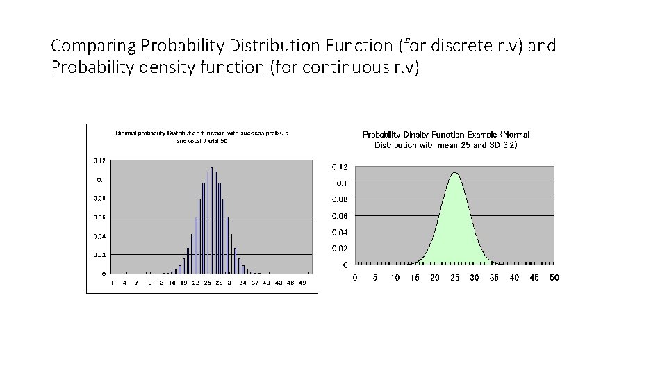
Comparing Probability Distribution Function (for discrete r. v) and Probability density function (for continuous r. v)

Continuous random variable A continuous random variable X has probability 0 for all outcomes!! Mathematically: P(X = x) = f(x) = 0 for all x Hence, we cannot represent the probability function f(x) by a table or bar chart as in the case of discrtete random variabes. Instead we use a continuous function – a density function. lecture 2 8

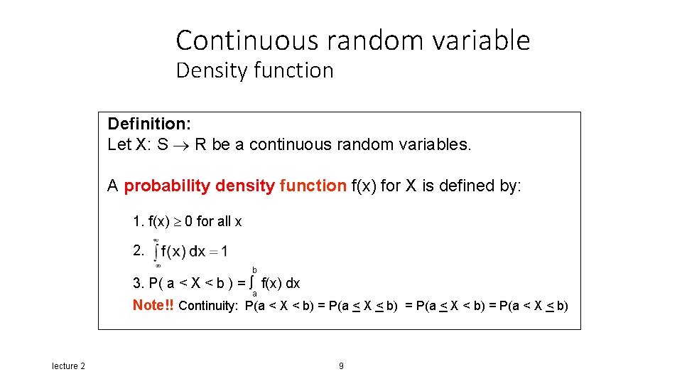
Continuous random variable Density function Definition: Let X: S R be a continuous random variables. A probability density function f(x) for X is defined by: 1. f(x) 0 for all x 2. b 3. P( a < X < b ) = f(x) dx a Note!! Continuity: P(a < X < b) = P(a < X < b) lecture 2 9

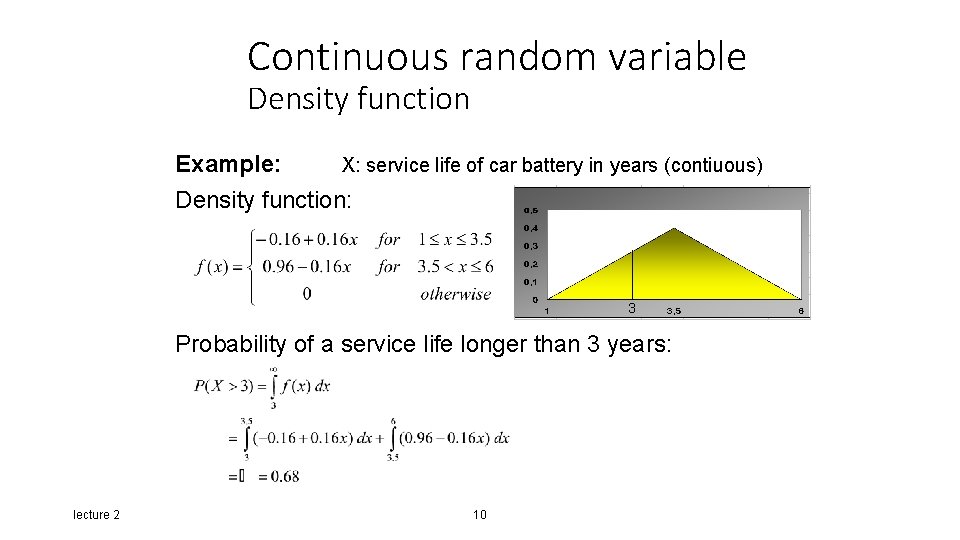
Continuous random variable Density function Example: X: service life of car battery in years (contiuous) Density function: 3 Probability of a service life longer than 3 years: lecture 2 10

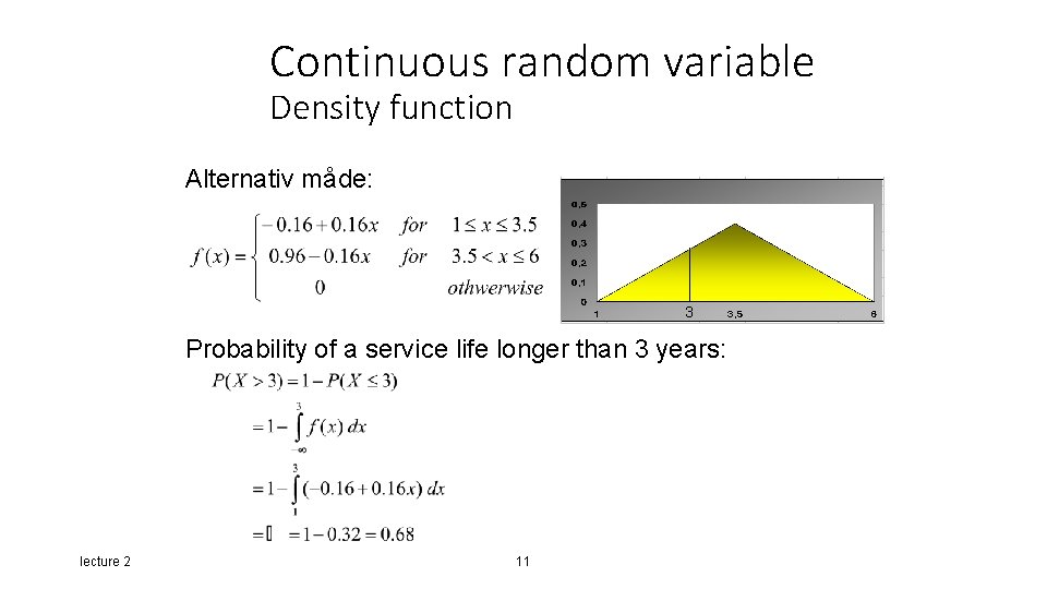
Continuous random variable Density function Alternativ måde: 3 Probability of a service life longer than 3 years: lecture 2 11

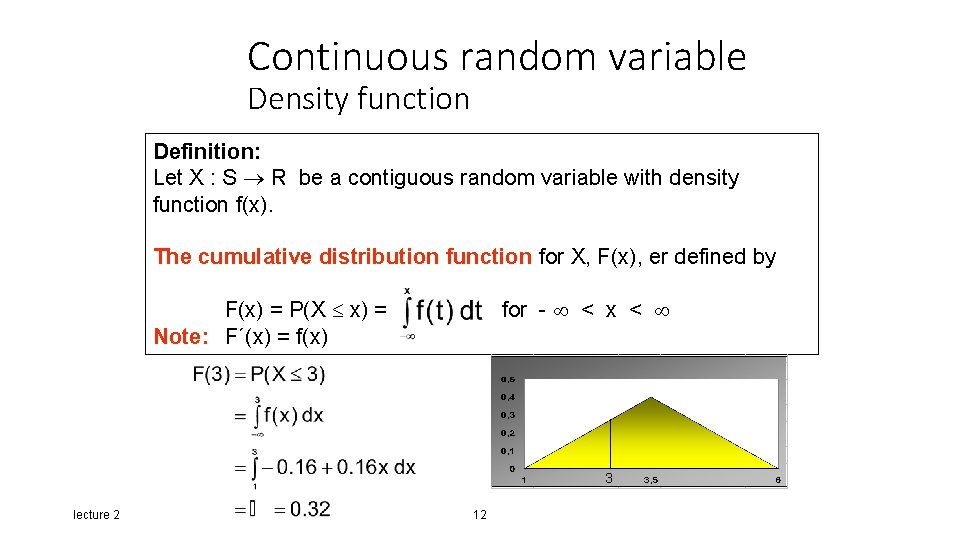
Continuous random variable Density function Definition: Let X : S R be a contiguous random variable with density function f(x). The cumulative distribution function for X, F(x), er defined by F(x) = P(X x) = Note: F´(x) = f(x) for - < x < 3 lecture 2 12

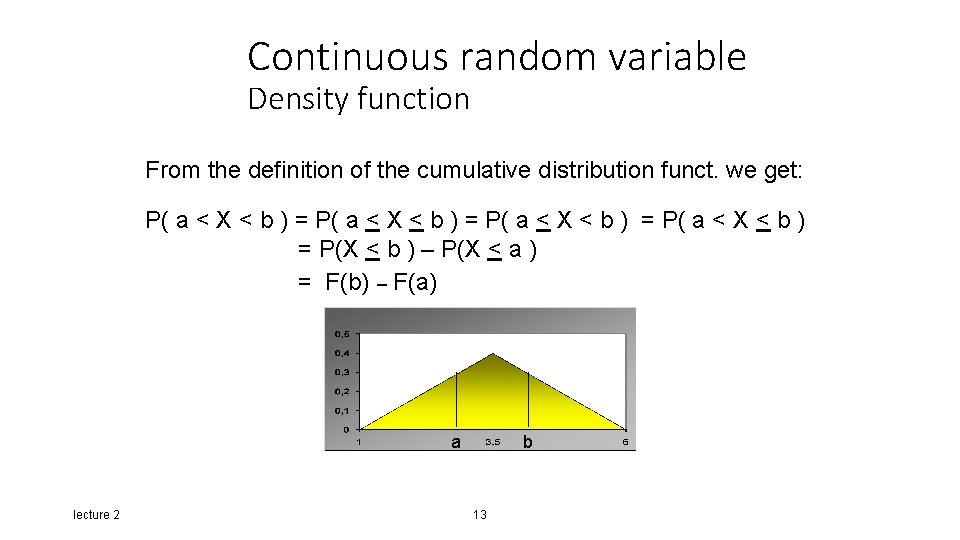
Continuous random variable Density function From the definition of the cumulative distribution funct. we get: P( a < X < b ) = P(X < b ) – P(X < a ) = F(b) – F(a) a lecture 2 b 13

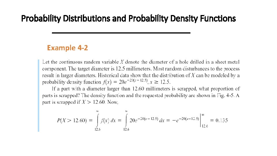
Probability Distributions and Probability Density Functions Example 4 -2

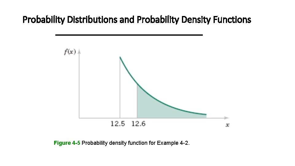
Probability Distributions and Probability Density Functions Figure 4 -5 Probability density function for Example 4 -2.

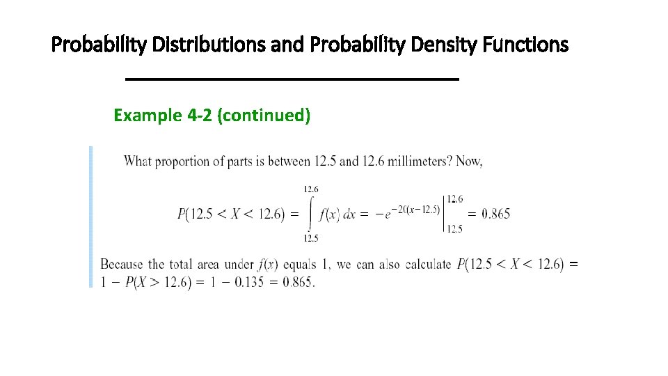
Probability Distributions and Probability Density Functions Example 4 -2 (continued)

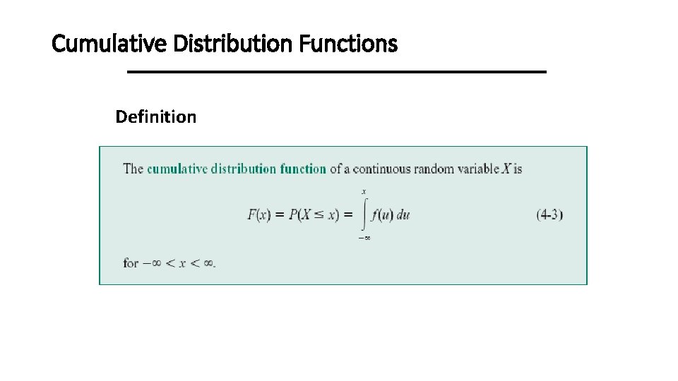
Cumulative Distribution Functions Definition

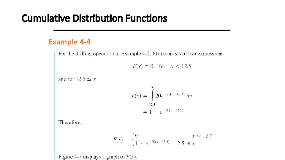
Cumulative Distribution Functions Example 4 -4

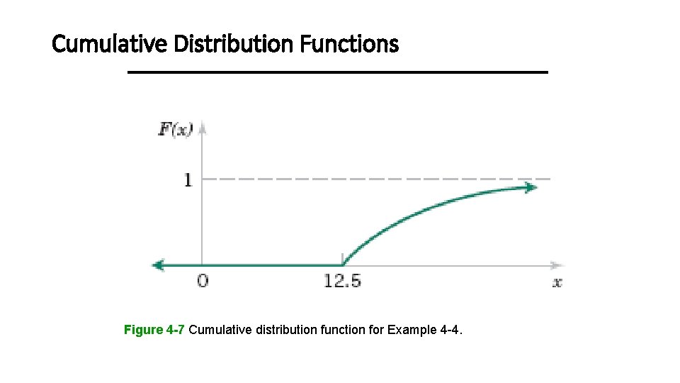
Cumulative Distribution Functions Figure 4 -7 Cumulative distribution function for Example 4 -4.

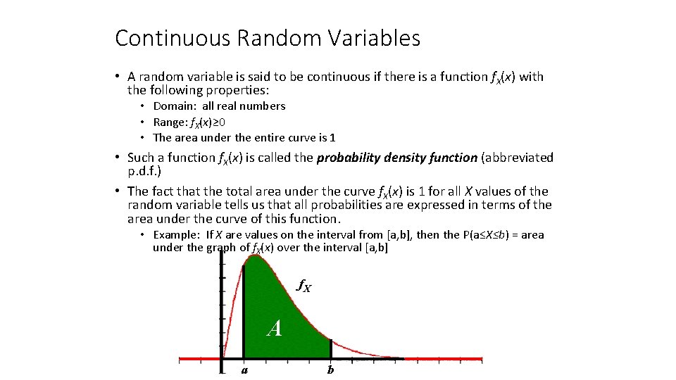
Continuous Random Variables • A random variable is said to be continuous if there is a function f. X(x) with the following properties: • Domain: all real numbers • Range: f. X(x)≥ 0 • The area under the entire curve is 1 • Such a function f. X(x) is called the probability density function (abbreviated p. d. f. ) • The fact that the total area under the curve f. X(x) is 1 for all X values of the random variable tells us that all probabilities are expressed in terms of the area under the curve of this function. • Example: If X are values on the interval from [a, b], then the P(a≤X≤b) = area under the graph of f. X(x) over the interval [a, b] f. X A a b

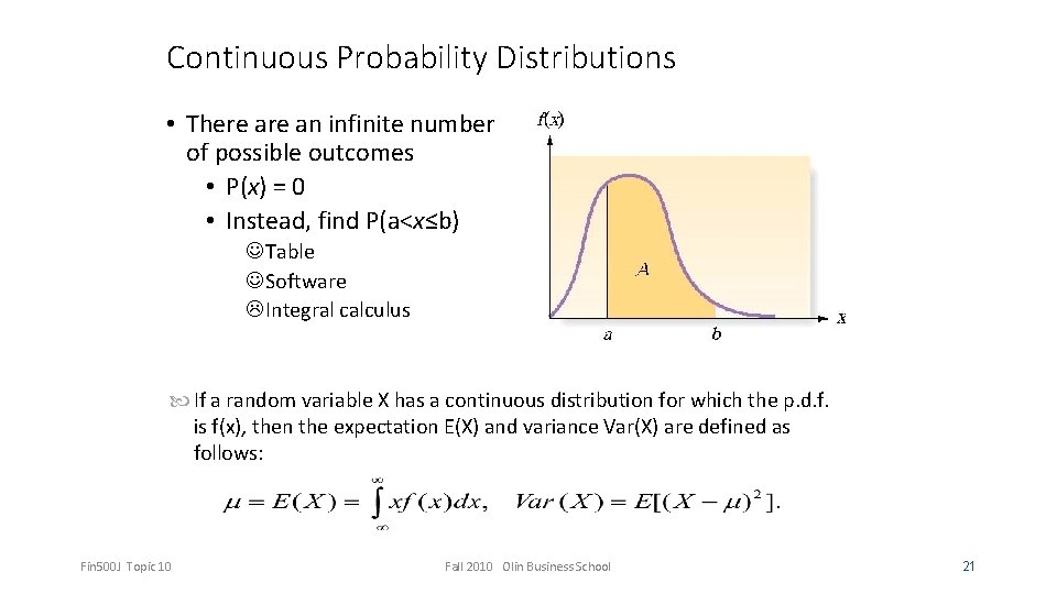
Continuous Probability Distributions • There an infinite number of possible outcomes • P(x) = 0 • Instead, find P(a<x≤b) Table Software Integral calculus If a random variable X has a continuous distribution for which the p. d. f. is f(x), then the expectation E(X) and variance Var(X) are defined as follows: Fin 500 J Topic 10 Fall 2010 Olin Business School 21

Uniform Random Variables: pdf • We want to define a random variable X that is “equally likely” to take on any value in some finite interval (a, b). Formally this is nonsensical since the probability of a continuous random variable assuming a particular value is always 0. A better way of formalizing our intuition is that the probability of X falling in a subinterval of (a, b) should depend only on the length of the subinterval, not on its location within (a, b). 11/5/2003 Probability and Statistics for Teachers, Math 507, Lecture 10 22

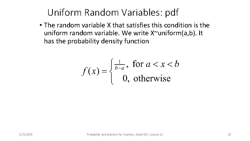
Uniform Random Variables: pdf • The random variable X that satisfies this condition is the uniform random variable. We write X~uniform(a, b). It has the probability density function 11/5/2003 Probability and Statistics for Teachers, Math 507, Lecture 10 23

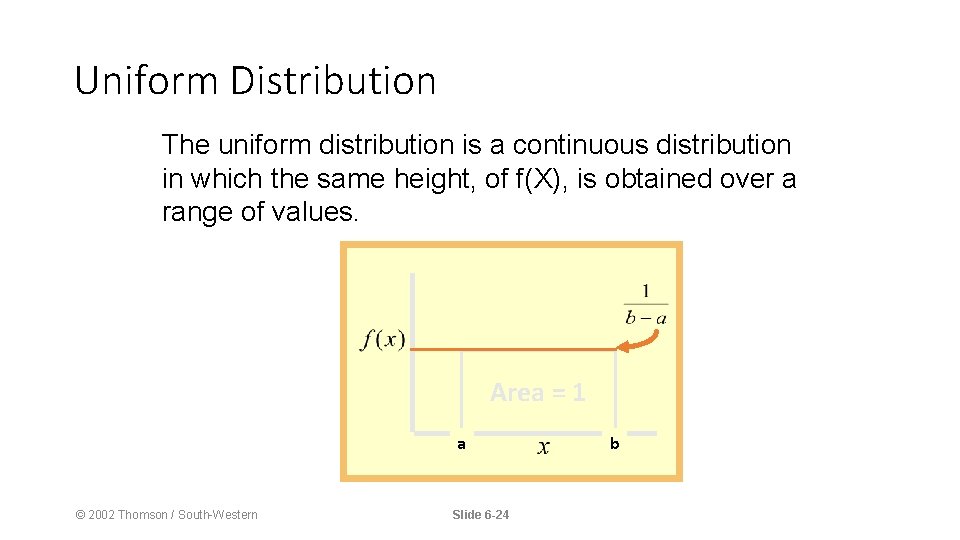
Uniform Distribution The uniform distribution is a continuous distribution in which the same height, of f(X), is obtained over a range of values. Area = 1 a © 2002 Thomson / South-Western Slide 6 -24 b

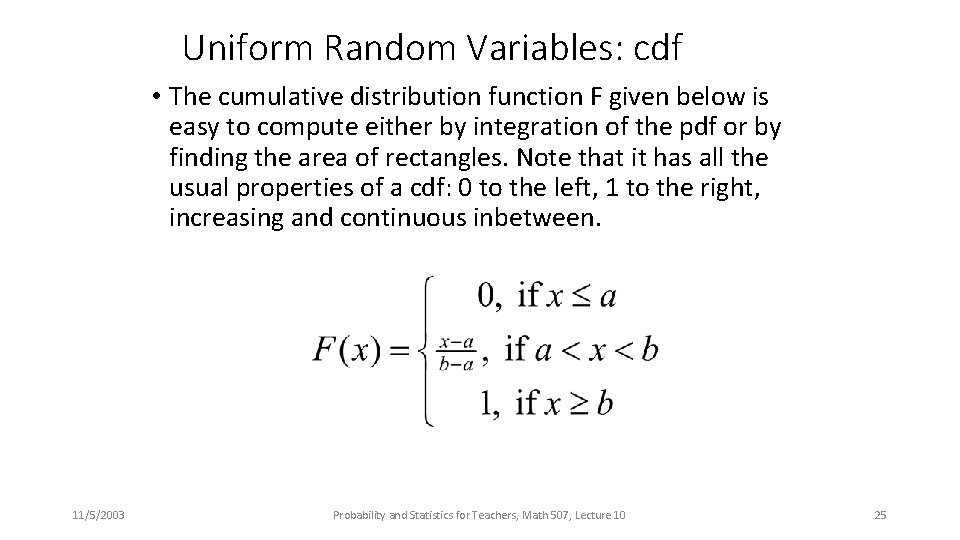
Uniform Random Variables: cdf • The cumulative distribution function F given below is easy to compute either by integration of the pdf or by finding the area of rectangles. Note that it has all the usual properties of a cdf: 0 to the left, 1 to the right, increasing and continuous inbetween. 11/5/2003 Probability and Statistics for Teachers, Math 507, Lecture 10 25

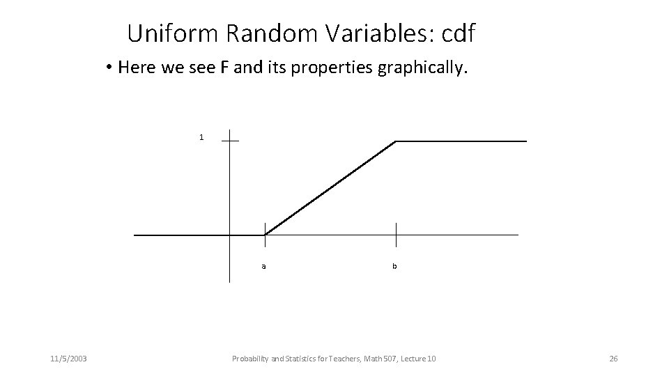
Uniform Random Variables: cdf • Here we see F and its properties graphically. 1 a 11/5/2003 b Probability and Statistics for Teachers, Math 507, Lecture 10 26

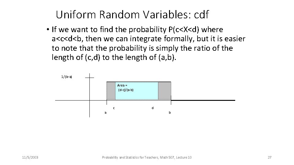
Uniform Random Variables: cdf • If we want to find the probability P(c<X<d) where a<c<d<b, then we can integrate formally, but it is easier to note that the probability is simply the ratio of the length of (c, d) to the length of (a, b). 1/(b-a) Area = (d-c)/(a-b) a 11/5/2003 c d b Probability and Statistics for Teachers, Math 507, Lecture 10 27

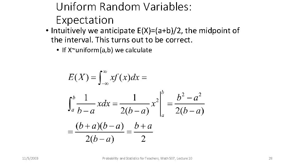
Uniform Random Variables: Expectation • Intuitively we anticipate E(X)=(a+b)/2, the midpoint of the interval. This turns out to be correct. • If X~uniform(a, b) we calculate 11/5/2003 Probability and Statistics for Teachers, Math 507, Lecture 10 28

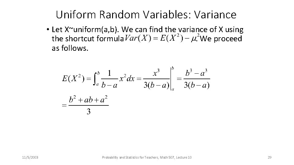
Uniform Random Variables: Variance • Let X~uniform(a, b). We can find the variance of X using the shortcut formula. We proceed as follows. 11/5/2003 Probability and Statistics for Teachers, Math 507, Lecture 10 29

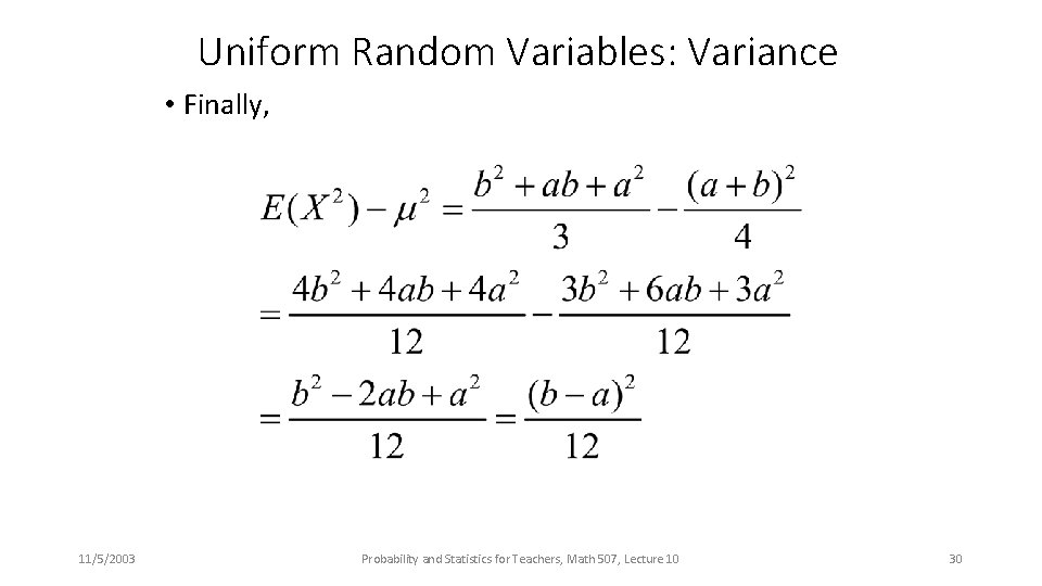
Uniform Random Variables: Variance • Finally, 11/5/2003 Probability and Statistics for Teachers, Math 507, Lecture 10 30

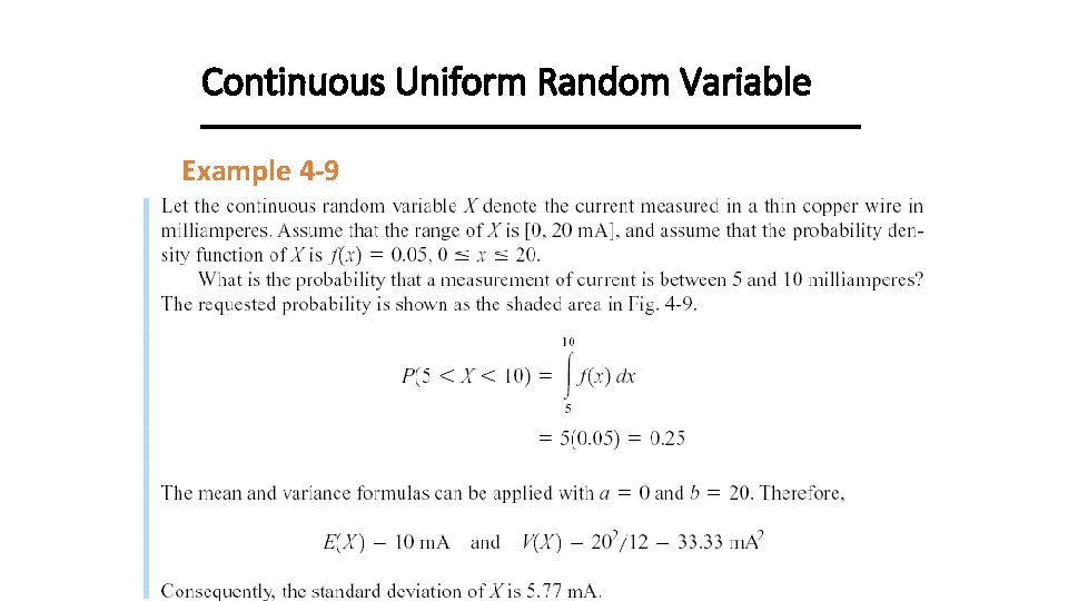
Continuous Uniform Random Variable Example 4 -9

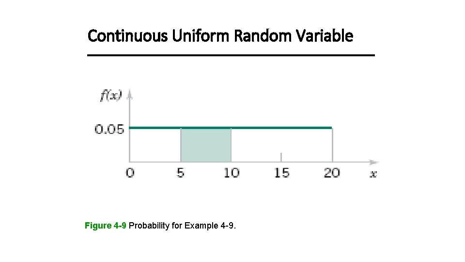
Continuous Uniform Random Variable Figure 4 -9 Probability for Example 4 -9.

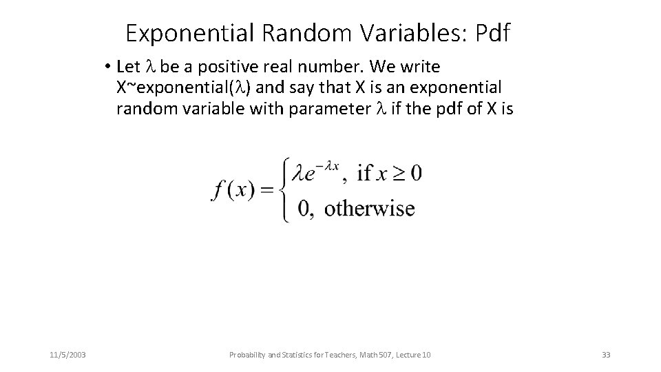
Exponential Random Variables: Pdf • Let be a positive real number. We write X~exponential( ) and say that X is an exponential random variable with parameter if the pdf of X is 11/5/2003 Probability and Statistics for Teachers, Math 507, Lecture 10 33

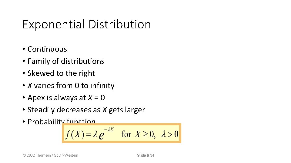
Exponential Distribution • Continuous • Family of distributions • Skewed to the right • X varies from 0 to infinity • Apex is always at X = 0 • Steadily decreases as X gets larger • Probability function © 2002 Thomson / South-Western Slide 6 -34

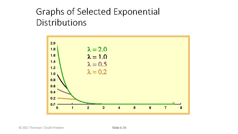
Graphs of Selected Exponential Distributions 2. 0 1. 8 1. 6 1. 4 1.

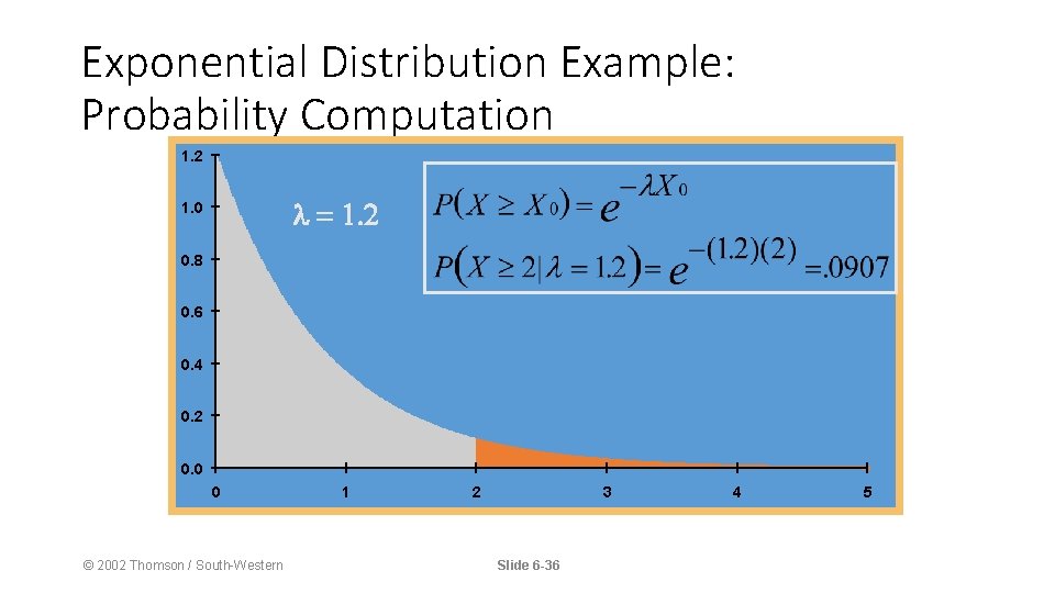
Exponential Distribution Example: Probability Computation 1. 2 1. 0 0. 8 0. 6 0.

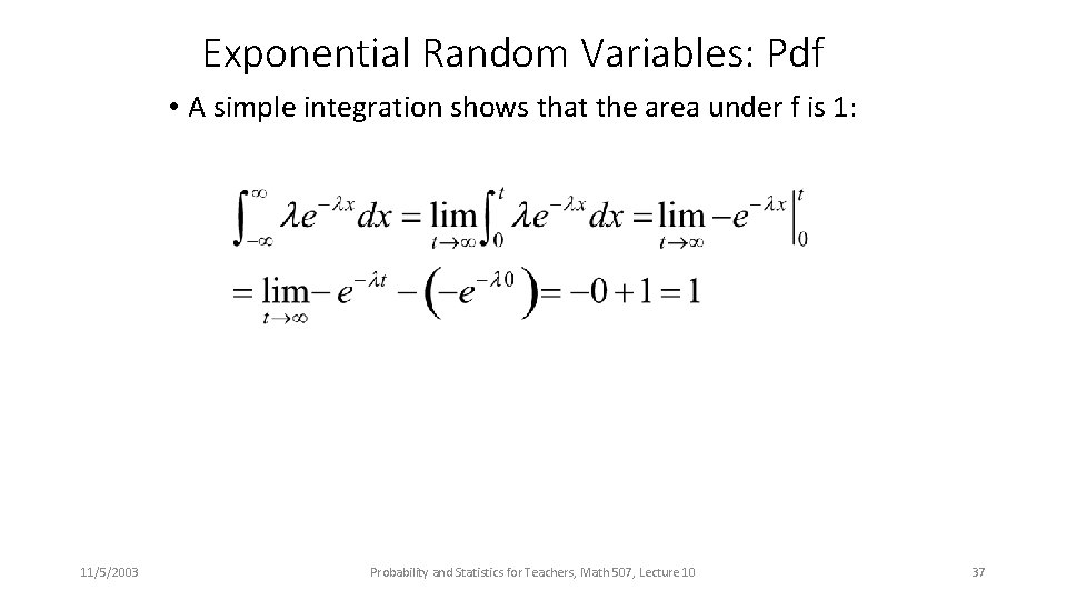
Exponential Random Variables: Pdf • A simple integration shows that the area under f is 1: 11/5/2003 Probability and Statistics for Teachers, Math 507, Lecture 10 37

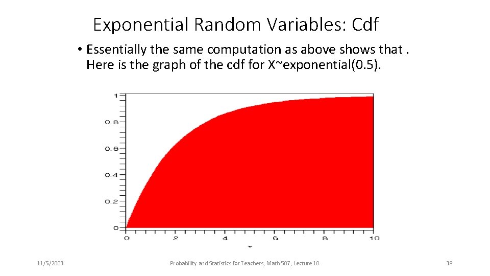
Exponential Random Variables: Cdf • Essentially the same computation as above shows that. Here is the graph of the cdf for X~exponential(0. 5). 11/5/2003 Probability and Statistics for Teachers, Math 507, Lecture 10 38

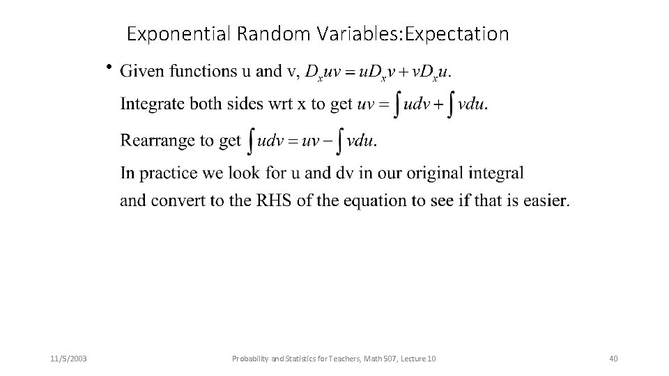
Exponential Random Variables: Expectation • Finding the expected value of X~exponential( ) is not hard as long as we remember how to integrate by parts. Recall that you can derive the integration by parts formula by differentiating a product of functions by the product rule, integrating both sides of the equation, and then rearranging algebraically. Thus integration by parts is the product rule used backwards and sideways. 11/5/2003 Probability and Statistics for Teachers, Math 507, Lecture 10 39

Exponential Random Variables: Expectation • 11/5/2003 Probability and Statistics for Teachers, Math 507, Lecture 10 40

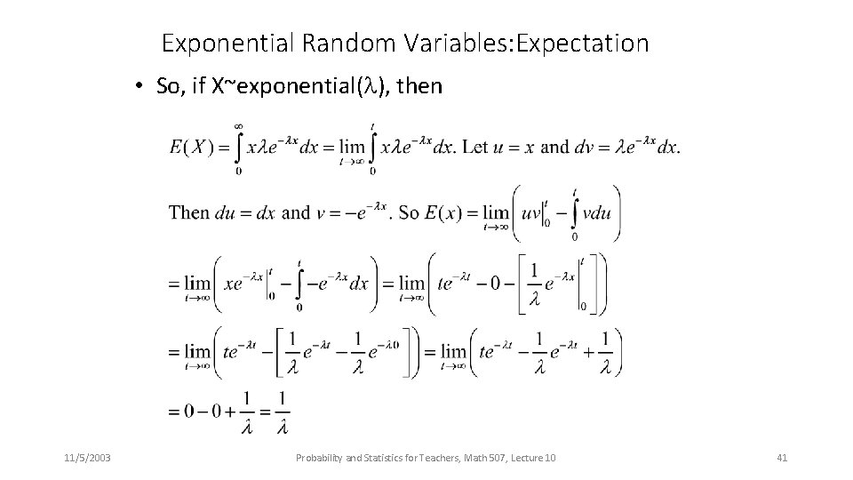
Exponential Random Variables: Expectation • So, if X~exponential( ), then 11/5/2003 Probability and Statistics for Teachers, Math 507, Lecture 10 41

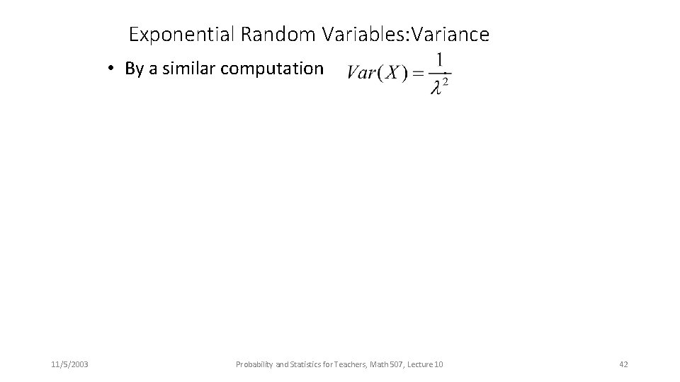
Exponential Random Variables: Variance • By a similar computation 11/5/2003 . Probability and Statistics for Teachers, Math 507, Lecture 10 42

Exponential Random Variables: Applications • Exponential distributions are sometimes used to model waiting times or lifetimes. That is, they model the time until some event happens or something quits working. Of course mathematics cannot tell us that exponentials are right to describe such situation. That conclusion depends on finding data from such real-world situations and fitting it to an exponential distribution. . 11/5/2003 Probability and Statistics for Teachers, Math 507, Lecture 10 43

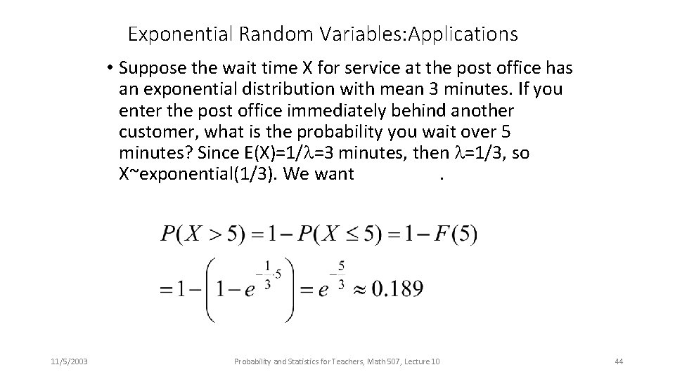
Exponential Random Variables: Applications • Suppose the wait time X for service at the post office has an exponential distribution with mean 3 minutes. If you enter the post office immediately behind another customer, what is the probability you wait over 5 minutes? Since E(X)=1/ =3 minutes, then =1/3, so X~exponential(1/3). We want. 11/5/2003 Probability and Statistics for Teachers, Math 507, Lecture 10 44

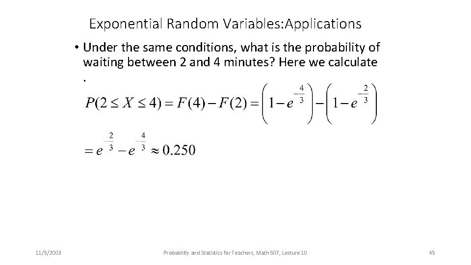
Exponential Random Variables: Applications • Under the same conditions, what is the probability of waiting between 2 and 4 minutes? Here we calculate. 11/5/2003 Probability and Statistics for Teachers, Math 507, Lecture 10 45

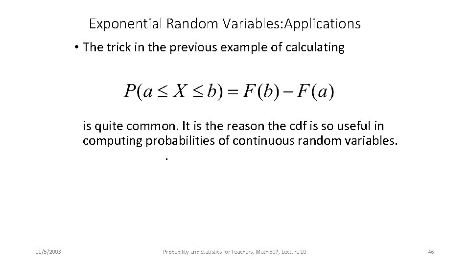
Exponential Random Variables: Applications • The trick in the previous example of calculating is quite common. It is the reason the cdf is so useful in computing probabilities of continuous random variables. . 11/5/2003 Probability and Statistics for Teachers, Math 507, Lecture 10 46

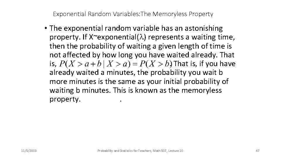
Exponential Random Variables: The Memoryless Property • The exponential random variable has an astonishing property. If X~exponential( ) represents a waiting time, then the probability of waiting a given length of time is not affected by how long you have waited already. That is, if you have already waited a minutes, the probability you wait b more minutes is the same as your initial probability of waiting b minutes. This is known as the memoryless property. . 11/5/2003 Probability and Statistics for Teachers, Math 507, Lecture 10 47

Exponential Random Variables: The Memoryless Property • Suppose you enter the post office and have to choose one of two lines, each of which has exactly one person ahead of you. The person in the first line got there just ahead of you. The person in the second line has already been there 10 minutes. Which line should you get in so as to be served fastest? If the waiting times are exponential, it does not matter. Similarly, if you are waiting for someone to get off a pay phone and you want to calculate the probability you have to wait more than 5 minutes, it is irrelevant to your calculations to know how long the person has already been on the phone. 11/5/2003 Probability and Statistics for Teachers, Math 507, Lecture 10 48

Exponential Random Variables: The Memoryless Property • In this respect exponential random variables behave like geometric ones. If you are finding the probability that, starting now, you flip a coin four times before getting heads, it is irrelevant to know how many times the coin flipped tails beforehand. 11/5/2003 Probability and Statistics for Teachers, Math 507, Lecture 10 49

The Normal Distribution • A widely known and much-used distribution that fits the measurements of many human characteristics and most machineproduced items. Many other variable in business and industry are normally distributed. • The normal distribution and its associated probabilities are an integral part of statistical quality control • Thus the normal distribution is the most important of all probability distributions. © 2002 Thomson / South-Western Slide 6 -50

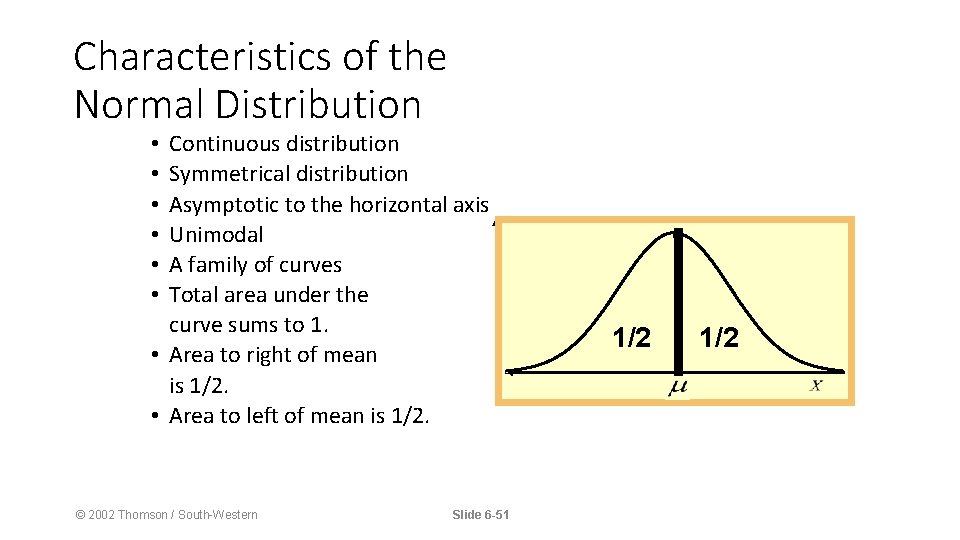
Characteristics of the Normal Distribution Continuous distribution Symmetrical distribution Asymptotic to the horizontal axis Unimodal A family of curves Total area under the curve sums to 1. • Area to right of mean is 1/2. • Area to left of mean is 1/2. • • • © 2002 Thomson / South-Western Slide 6 -51 1/2

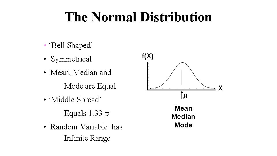
The Normal Distribution • ‘Bell Shaped’ • Symmetrical f(X) • Mean, Median and Mode are Equal • ‘Middle Spread’ Equals 1. 33 • Random Variable has Infinite Range Mean Median Mode X

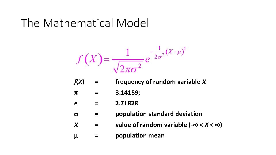
The Mathematical Model f(X) = frequency of random variable X = 3. 14159; e = 2. 71828 = population standard deviation X = value of random variable (- < X < ) = population mean

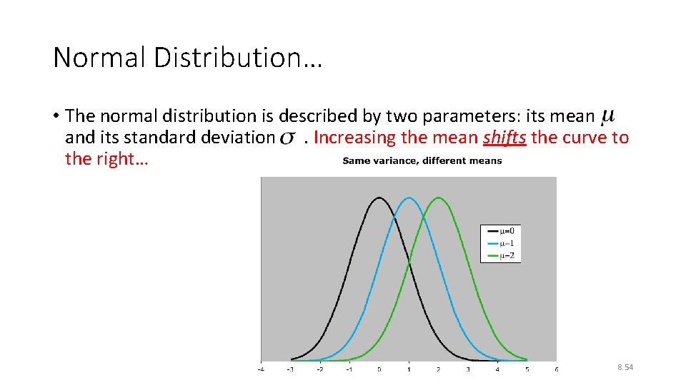
Normal Distribution… • The normal distribution is described by two parameters: its mean and its standard deviation. Increasing the mean shifts the curve to the right… 8. 54

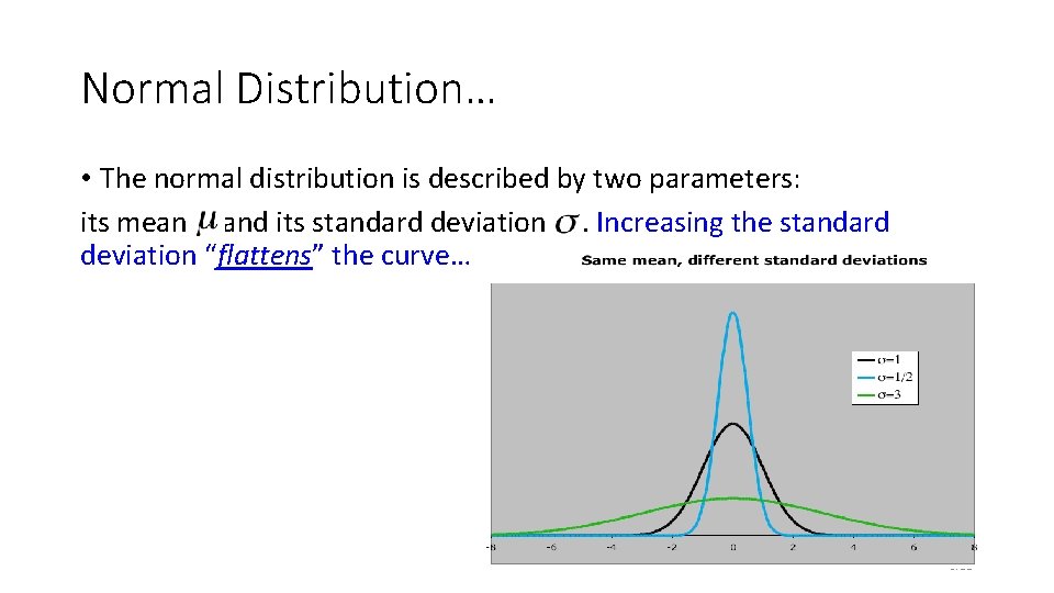
Normal Distribution… • The normal distribution is described by two parameters: its mean and its standard deviation. Increasing the standard deviation “flattens” the curve… 8. 55

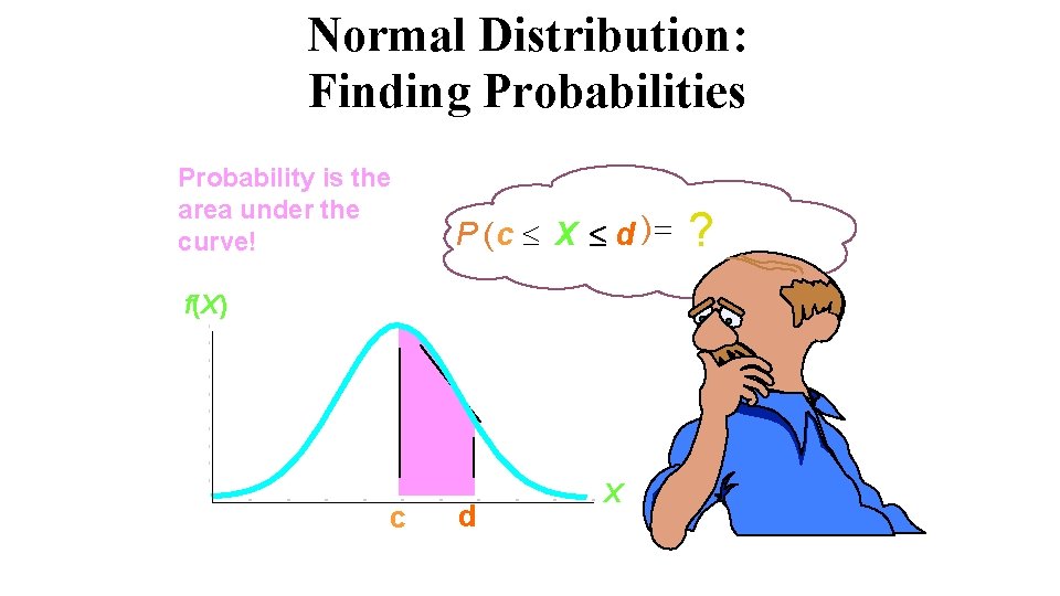
Normal Distribution: Finding Probabilities Probability is the area under the curve! P (c X d ) f(X) c d X ?

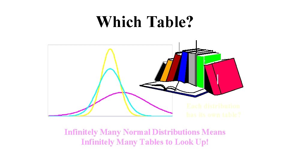
Which Table? Each distribution has its own table? Infinitely Many Normal Distributions Means Infinitely Many Tables to Look Up!

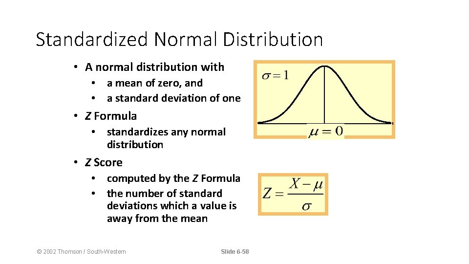
Standardized Normal Distribution • A normal distribution with • a mean of zero, and • a standard deviation of one • Z Formula • standardizes any normal distribution • Z Score • computed by the Z Formula • the number of standard deviations which a value is away from the mean © 2002 Thomson / South-Western Slide 6 -58

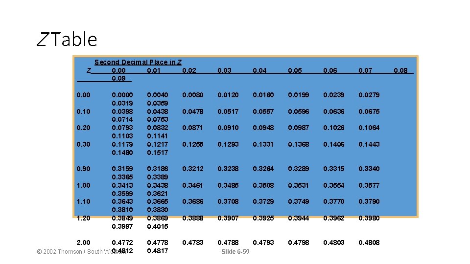
Z Table Second Decimal Place in Z Z 0. 00 0. 01 0. 02 0. 09 0. 00 0. 03 0. 04 0. 05 0. 06 0. 07 0. 0000 0. 0319 0. 0398 0. 0714 0. 0793 0. 1103 0. 1179 0. 1480 0. 0040 0. 0359 0. 0438 0. 0753 0. 0832 0. 1141 0. 1217 0. 1517 0. 0080 0. 0120 0. 0160 0. 0199 0. 0239 0. 0279 0. 0478 0. 0517 0. 0557 0. 0596 0. 0636 0. 0675 0. 0871 0. 0910 0. 0948 0. 0987 0. 1026 0. 1064 0. 1255 0. 1293 0. 1331 0. 1368 0. 1406 0. 1443 0. 3159 0. 3365 0. 3413 0. 3599 0. 3643 0. 3810 0. 3849 0. 3997 0. 3186 0. 3389 0. 3438 0. 3621 0. 3665 0. 3830 0. 3869 0. 4015 0. 3212 0. 3238 0. 3264 0. 3289 0. 3315 0. 3340 0. 3461 0. 3485 0. 3508 0. 3531 0. 3554 0. 3577 0. 3686 0. 3708 0. 3729 0. 3749 0. 3770 0. 3790 0. 3888 0. 3907 0. 3925 0. 3944 0. 3962 0. 3980 0. 4772 0. 4812 © 2002 Thomson / South-Western 0. 4778 0. 4817 0. 4783 0. 4788 0. 4793 0. 4798 0. 4803 0. 4808 0. 10 0. 20 0. 30 0. 90 1. 00 1. 10 1. 20 2. 00 Slide 6 -59 0. 08

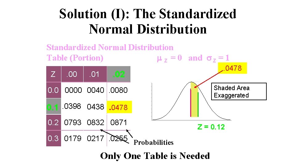
Solution (I): The Standardized Normal Distribution Table (Portion) Z = 0 and Z = 1 Z . 00 . 01 . 0478 . 02 Shaded Area Exaggerated 0. 0. 0000. 0040. 0080 0. 1. 0398. 0438. 0478 0. 2. 0793. 0832. 0871 Z = 0. 12 0. 3. 0179. 0217. 0255 Probabilities Only One Table is Needed

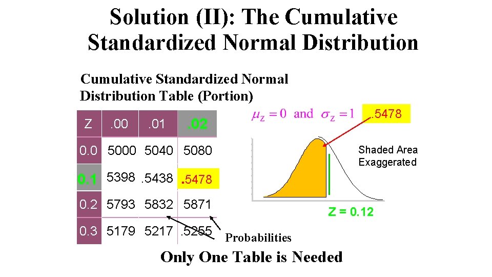
Solution (II): The Cumulative Standardized Normal Distribution Table (Portion) Z . 00 . 01 . 5478 . 02 0. 0. 5000. 5040. 5080 Shaded Area Exaggerated 0. 1. 5398. 5438. 5478 0. 2. 5793. 5832. 5871 0. 3. 5179. 5217. 5255 Z = 0. 12 Probabilities Only One Table is Needed

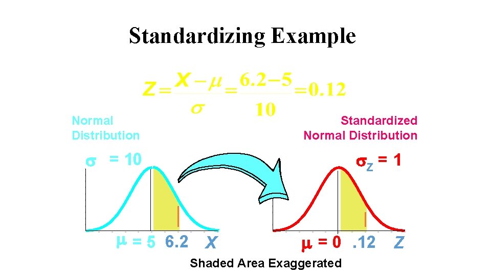
Standardizing Example Normal Distribution Standardized Normal Distribution = 10 Z = 1 = 5 6. 2 X = 0. 12 Shaded Area Exaggerated Z

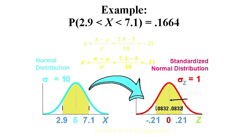
Example: P(2. 9 < X < 7. 1) =. 1664 Normal Distribution Standardized Normal Distribution = 10 Z = 1. 1664. 0832 2. 9 5 7. 1 X -. 21 0. 21 Shaded Area Exaggerated Z

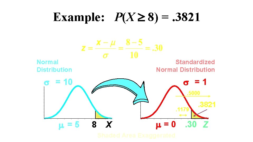
Example: P(X 8) =. 3821. Normal Distribution Standardized Normal Distribution = 10 =1. 5000. 1179 =5 8 X . 3821 = 0. 30 Z Shaded Area Exaggerated

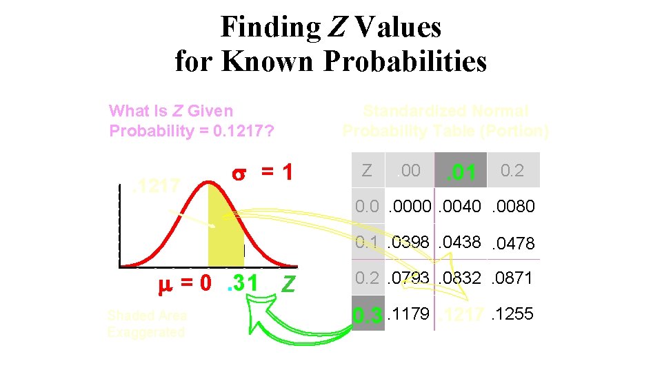
Finding Z Values for Known Probabilities What Is Z Given Probability = 0. 1217? . 1217 =1 Standardized Normal Probability Table (Portion) Z . 00 . 01 0. 2 0. 0. 0000. 0040. 0080 0. 1. 0398. 0438. 0478 = 0. 31 Z Shaded Area Exaggerated 0. 2. 0793. 0832. 0871 0. 3. 1179. 1217. 1255

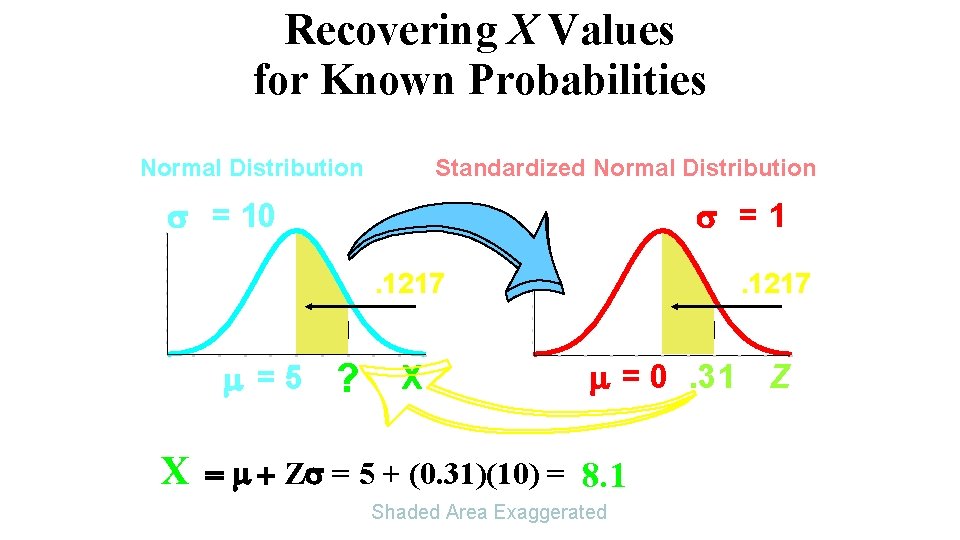
Recovering X Values for Known Probabilities Normal Distribution Standardized Normal Distribution = 10 =1. 1217 =5 ? X . 1217 = 0. 31 X Z = 5 + (0. 31)(10) = 8. 1 Shaded Area Exaggerated Z

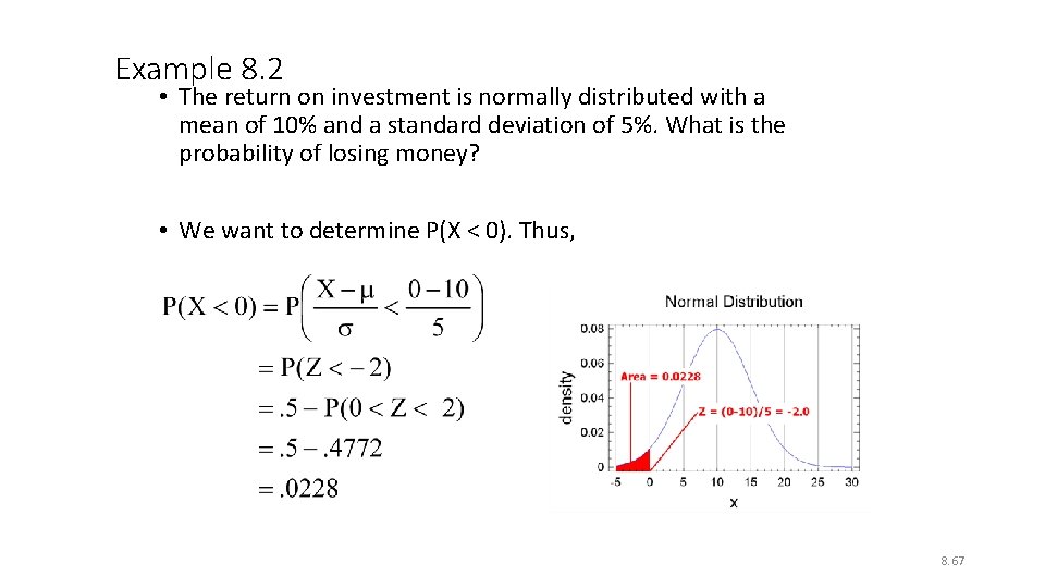
Example 8. 2 • The return on investment is normally distributed with a mean of 10% and a standard deviation of 5%. What is the probability of losing money? • We want to determine P(X < 0). Thus, 8. 67

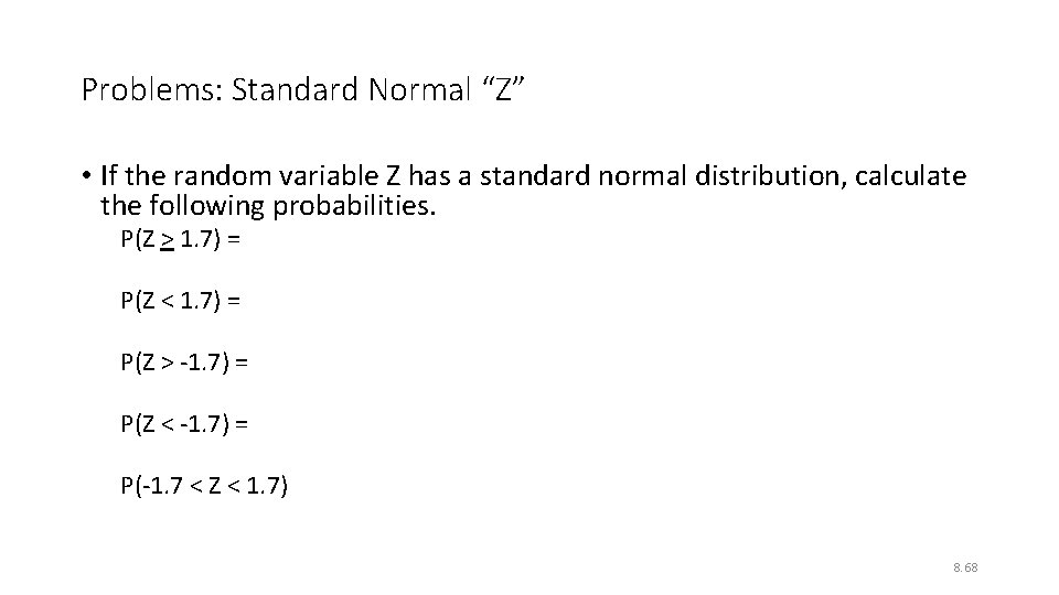
Problems: Standard Normal “Z” • If the random variable Z has a standard normal distribution, calculate the following probabilities. P(Z > 1. 7) = P(Z < 1. 7) = P(Z > -1. 7) = P(Z < -1. 7) = P(-1. 7 < Z < 1. 7) 8. 68

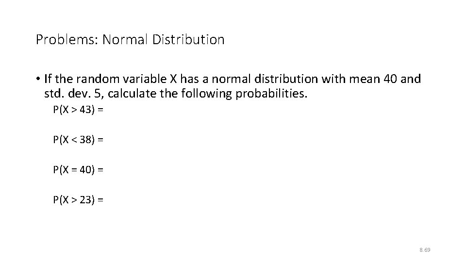
Problems: Normal Distribution • If the random variable X has a normal distribution with mean 40 and std. dev. 5, calculate the following probabilities. P(X > 43) = P(X < 38) = P(X = 40) = P(X > 23) = 8. 69

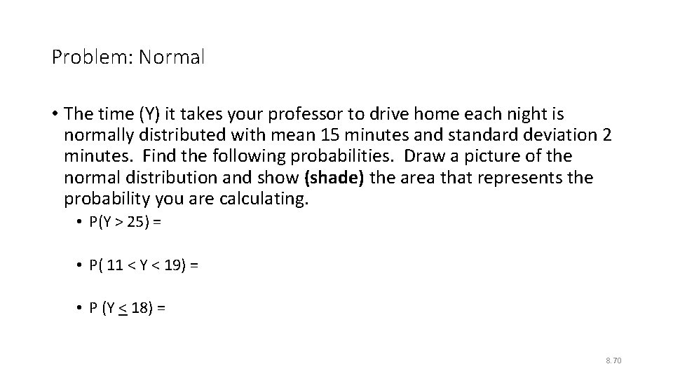
Problem: Normal • The time (Y) it takes your professor to drive home each night is normally distributed with mean 15 minutes and standard deviation 2 minutes. Find the following probabilities. Draw a picture of the normal distribution and show (shade) the area that represents the probability you are calculating. • P(Y > 25) = • P( 11 < Y < 19) = • P (Y < 18) = 8. 70

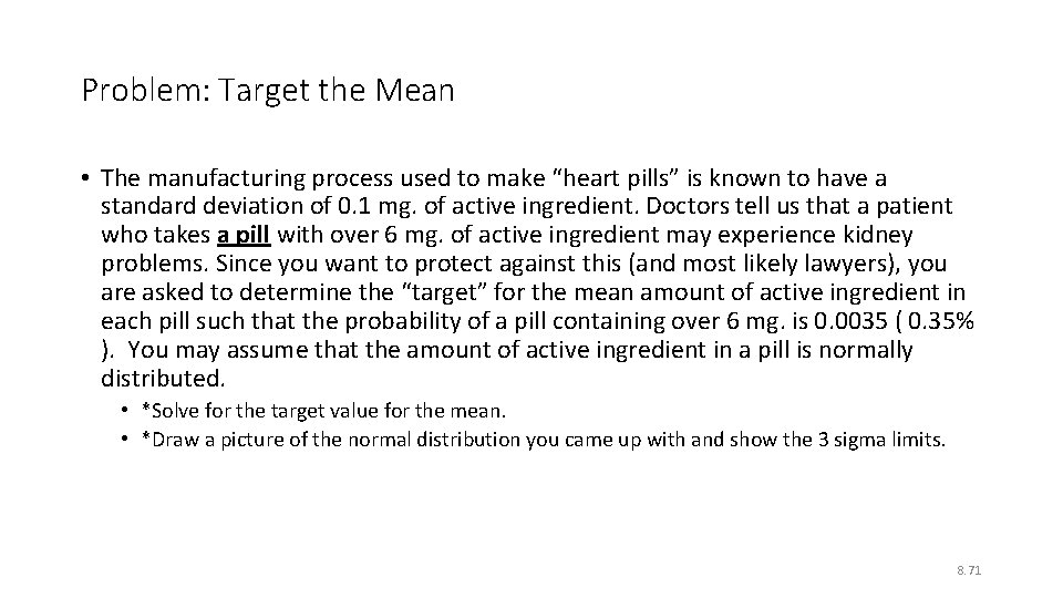
Problem: Target the Mean • The manufacturing process used to make “heart pills” is known to have a standard deviation of 0. 1 mg. of active ingredient. Doctors tell us that a patient who takes a pill with over 6 mg. of active ingredient may experience kidney problems. Since you want to protect against this (and most likely lawyers), you are asked to determine the “target” for the mean amount of active ingredient in each pill such that the probability of a pill containing over 6 mg. is 0. 0035 ( 0. 35% ). You may assume that the amount of active ingredient in a pill is normally distributed. • *Solve for the target value for the mean. • *Draw a picture of the normal distribution you came up with and show the 3 sigma limits. 8. 71