Random variables continued 1 Repeated measurements student scientists

Random variables (continued) 1

Repeated measurements student scientists are taught to perform multiple measurements and average the results one reason is to increase the precision of the estimated value if taking multiple measurements increases the precision then surely taking even more measurements would be better? how does the precision of the average behave as a function of the number of measurements n? 2

Variance of the mean precision = variance (or standard deviation) assume the measurement is contaminated with additive Gaussian noise with mean zero and variance 1 write a simulation to study the behavior of the sample mean as a function of the number of measurements 3

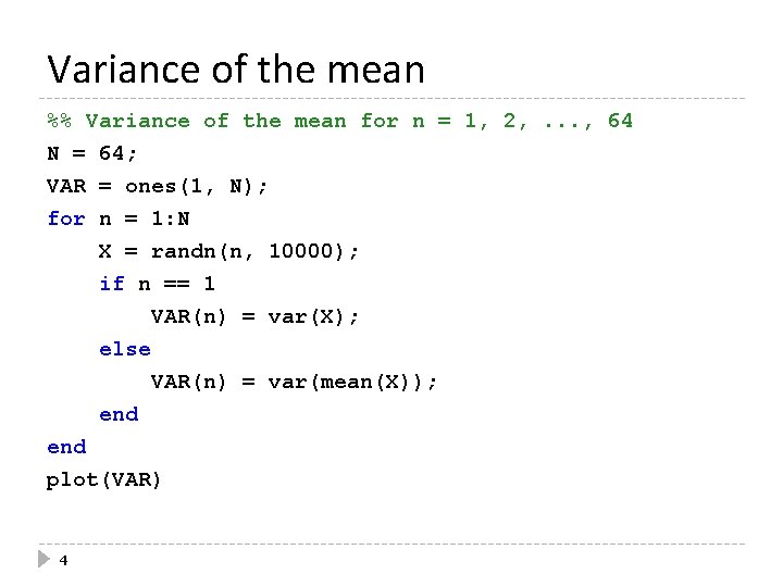
Variance of the mean %% Variance of the mean for n = 1, 2, . . . , 64 N = 64; VAR = ones(1, N); for n = 1: N X = randn(n, 10000); if n == 1 VAR(n) = var(X); else VAR(n) = var(mean(X)); end plot(VAR) 4

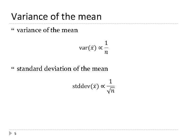
Variance of the mean variance of the mean standard deviation of the mean 5

Gaussian random walk a Gaussian random walk is a random walk where the step size is drawn from a Gaussian distribution with mean variance 6

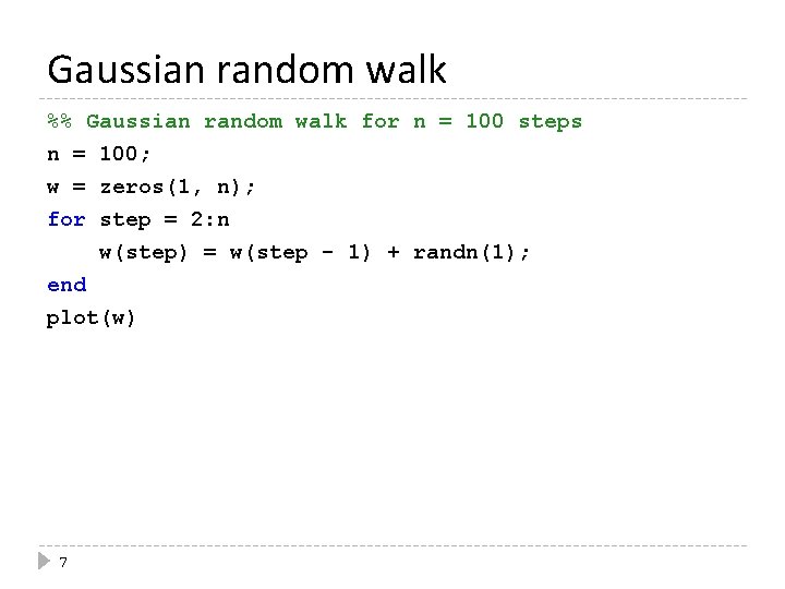
Gaussian random walk %% Gaussian random walk for n = 100 steps n = 100; w = zeros(1, n); for step = 2: n w(step) = w(step - 1) + randn(1); end plot(w) 7

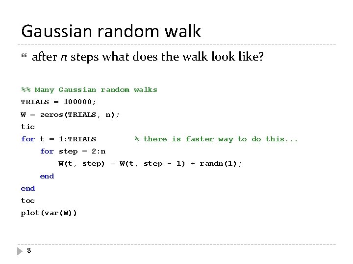
Gaussian random walk after n steps what does the walk look like? %% Many Gaussian random walks TRIALS = 100000; W = zeros(TRIALS, n); tic for t = 1: TRIALS % there is faster way to do this. . . for step = 2: n W(t, step) = W(t, step - 1) + randn(1); end toc plot(var(W)) 8

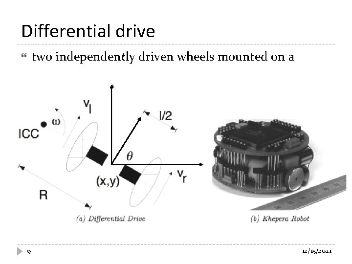
Differential drive two independently driven wheels mounted on a common axis 9 12/15/2021

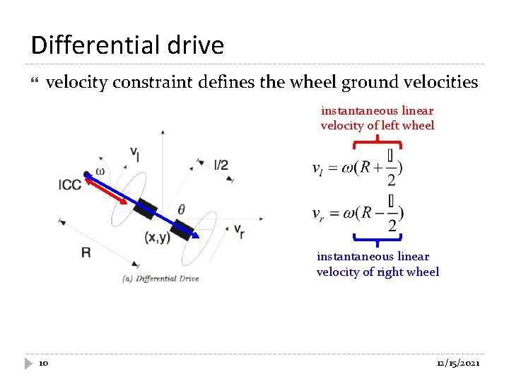
Differential drive velocity constraint defines the wheel ground velocities instantaneous linear velocity of left wheel instantaneous linear velocity of right wheel 10 12/15/2021

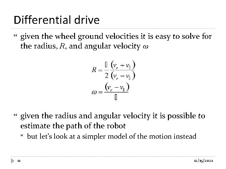
Differential drive given the wheel ground velocities it is easy to solve for the radius, R, and angular velocity ω given the radius and angular velocity it is possible to estimate the path of the robot 11 but let's look at a simpler model of the motion instead 12/15/2021

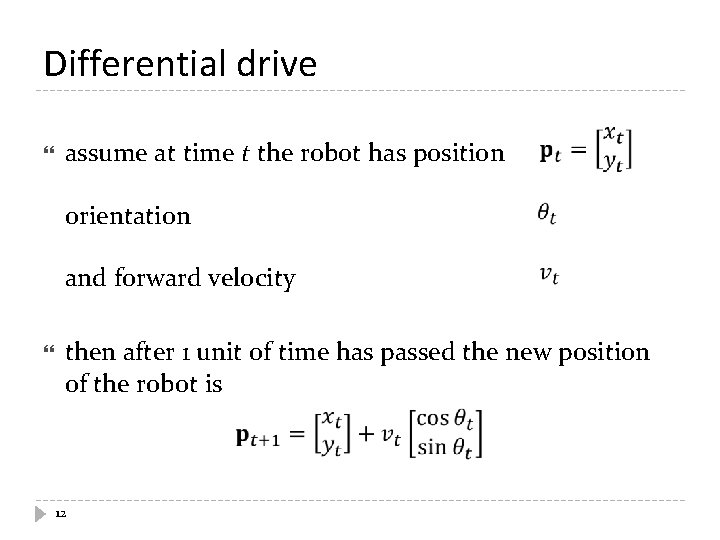
Differential drive assume at time t the robot has position orientation and forward velocity then after 1 unit of time has passed the new position of the robot is 12

Differential drive 13

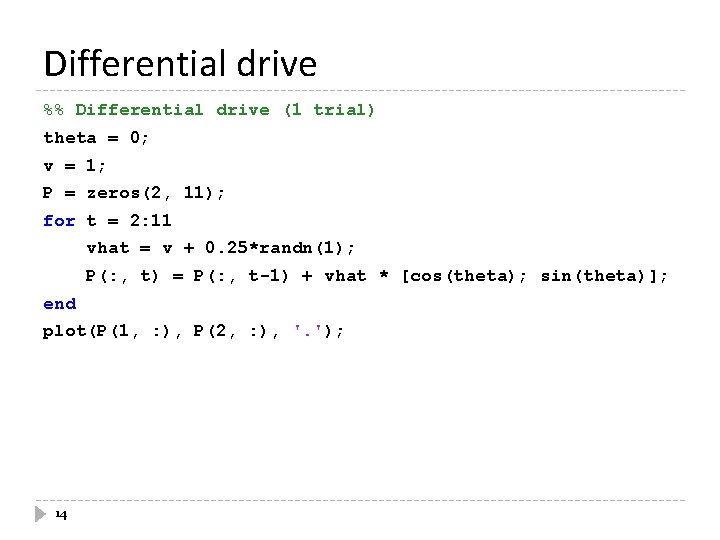
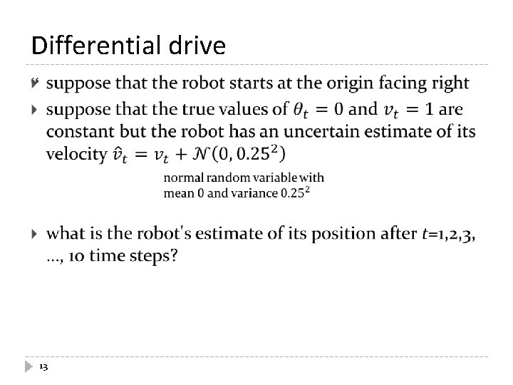
Differential drive %% Differential drive (1 trial) theta = 0; v = 1; P = zeros(2, 11); for t = 2: 11 vhat = v + 0. 25*randn(1); P(: , t) = P(: , t-1) + vhat * [cos(theta); sin(theta)]; end plot(P(1, : ), P(2, : ), '. '); 14

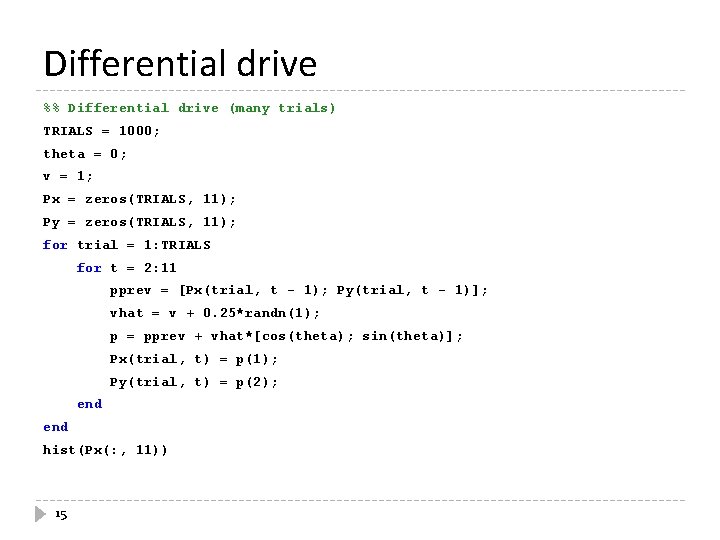
Differential drive %% Differential drive (many trials) TRIALS = 1000; theta = 0; v = 1; Px = zeros(TRIALS, 11); Py = zeros(TRIALS, 11); for trial = 1: TRIALS for t = 2: 11 pprev = [Px(trial, t - 1); Py(trial, t - 1)]; vhat = v + 0. 25*randn(1); p = pprev + vhat*[cos(theta); sin(theta)]; Px(trial, t) = p(1); Py(trial, t) = p(2); end hist(Px(: , 11)) 15

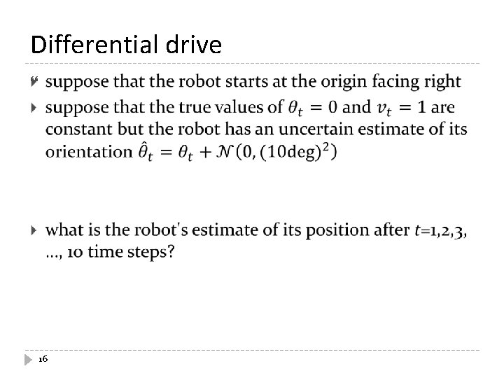
Differential drive 16

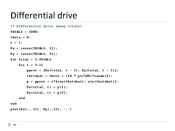
Differential drive %% Differential drive (many trials) TRIALS = 1000; theta = 0; v = 1; Px = zeros(TRIALS, 11); Py = zeros(TRIALS, 11); for trial = 1: TRIALS for t = 2: 11 pprev = [Px(trial, t - 1); Py(trial, t - 1)]; thetahat = theta + (10 * pi/180)*randn(1); p = pprev + v*[cos(thetahat); sin(thetahat)]; Px(trial, t) = p(1); Py(trial, t) = p(2); end plot(Px(: , 11), Py(: , 11), '. ') 17