Random Variables and Probability Distributions l A random

Random Variables and Probability Distributions l A random variable is a function or rule that assigns a numerical value to each simple event in a sample space. l 為了降低分析的複雜性，將所有可能結果加以數值化 例如投銅板十次，正面出現次數的事件就是random variable l 短期不知道是什麼，長期下來會呈現某種分配 l l There are two types of random variables: l l 2 Discrete random variable Continuous random variable

Discrete Probability Distribution l A table, formula, or graph that lists all possible values a discrete random variable can assume, together with associated probabilities, is called a discrete probability distribution. l To calculate the probability that the random variable X assumes the value x, P(X = x), l l l 3 add the probabilities of all the simple events for which X is equal to x, or Use probability calculation tools (tree diagram), Apply probability definitions

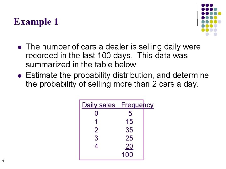
Example 1 l l The number of cars a dealer is selling daily were recorded in the last 100 days. This data was summarized in the table below. Estimate the probability distribution, and determine the probability of selling more than 2 cars a day. Daily sales Frequency 0 5 1 15 2 35 3 25 4 20 100 4

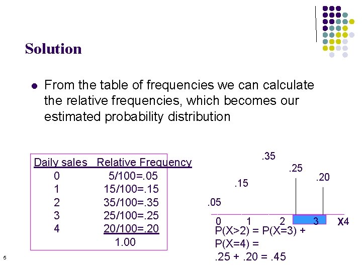
Solution l From the table of frequencies we can calculate the relative frequencies, which becomes our estimated probability distribution Daily sales Relative Frequency 0 5/100=. 05 1 15/100=. 15 2 35/100=. 35 3 25/100=. 25 4 20/100=. 20 1. 00 5 . 35. 25. 15 . 20 . 05 0 1 2 P(X>2) = P(X=3) + P(X=4) =. 25 +. 20 =. 45 3 X 4

Describing the Population/ Probability Distribution l l l 6 The probability distribution represents a population We’re interested in describing the population by computing various parameters. Specifically, we calculate the population mean and population variance.

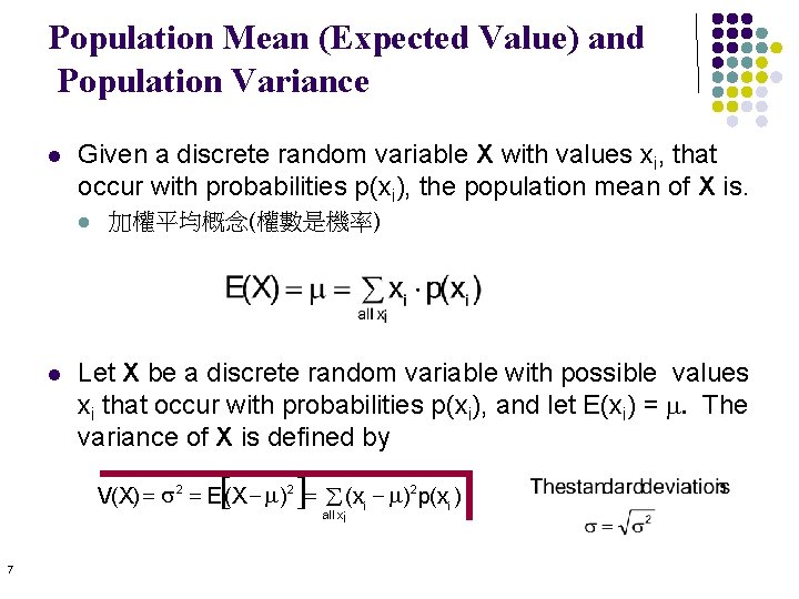
Population Mean (Expected Value) and Population Variance l Given a discrete random variable X with values xi, that occur with probabilities p(xi), the population mean of X is. l l 加權平均概念(權數是機率) Let X be a discrete random variable with possible values xi that occur with probabilities p(xi), and let E(xi) = m. The variance of X is defined by V(X) = s 2 = E[(X - m)2 ]= å (xi - m)2 p(xi ) all xi 7

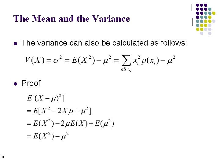
The Mean and the Variance 8 l The variance can also be calculated as follows: l Proof

Laws of Expected Value and Variance l Laws of Expected Value § § § l Laws of Variance § § § 9 E(c) = c E(X + c) = E(X) + c E(c. X) = c. E(X) V(c) = 0 V(X + c) = V(X) V(c. X) = c 2 V(X)

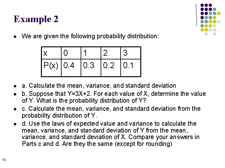
Example 2 l We are given the following probability distribution: x 0 P(x) 0. 4 l l 10 1 2 3 0. 2 0. 1 a. Calculate the mean, variance, and standard deviation b. Suppose that Y=3 X+2. For each value of X, determine the value of Y. What is the probability distribution of Y? c. Calculate the mean, variance, and standard deviation from the probability distribution of Y. d. Use the laws of expected value and variance to calculate the mean, variance, and standard deviation of Y from the mean, variance, and standard deviation of X. Compare your answers in Parts c and d. Are they the same (except for rounding)

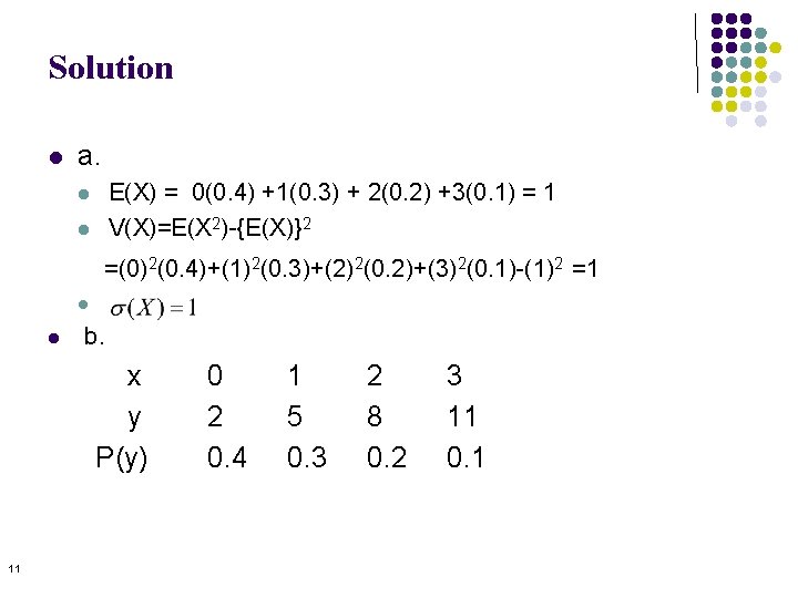
Solution l a. E(X) = 0(0. 4) +1(0. 3) + 2(0. 2) +3(0. 1) = 1 V(X)=E(X 2)-{E(X)}2 l l =(0)2(0. 4)+(1)2(0. 3)+(2)2(0. 2)+(3)2(0. 1)-(1)2 =1 l l b. x y P(y) 11 0 2 0. 4 1 5 0. 3 2 8 0. 2 3 11 0. 1

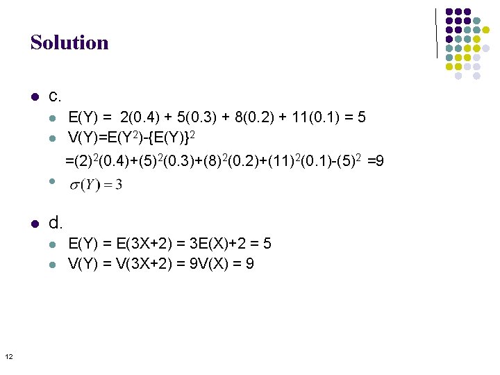
Solution l c. l l E(Y) = 2(0. 4) + 5(0. 3) + 8(0. 2) + 11(0. 1) = 5 V(Y)=E(Y 2)-{E(Y)}2 =(2)2(0. 4)+(5)2(0. 3)+(8)2(0. 2)+(11)2(0. 1)-(5)2 =9 l l d. l l 12 E(Y) = E(3 X+2) = 3 E(X)+2 = 5 V(Y) = V(3 X+2) = 9 V(X) = 9

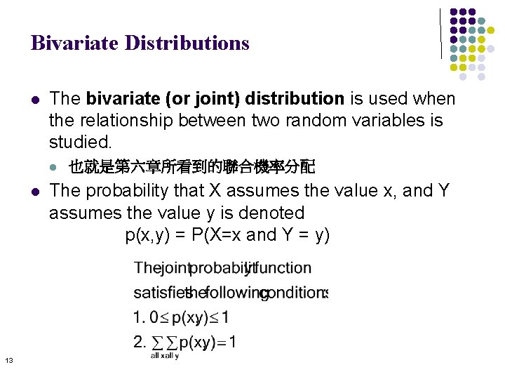
Bivariate Distributions l The bivariate (or joint) distribution is used when the relationship between two random variables is studied. l l 13 也就是第六章所看到的聯合機率分配 The probability that X assumes the value x, and Y assumes the value y is denoted p(x, y) = P(X=x and Y = y)

Bivariate Distributions l 14 Example 7. 5 l Xavier and Yvette are two real estate agents. Let X and Y denote the number of houses that Xavier and Yvette will sell next week, respectively. l The bivariate probability distribution is presented next.

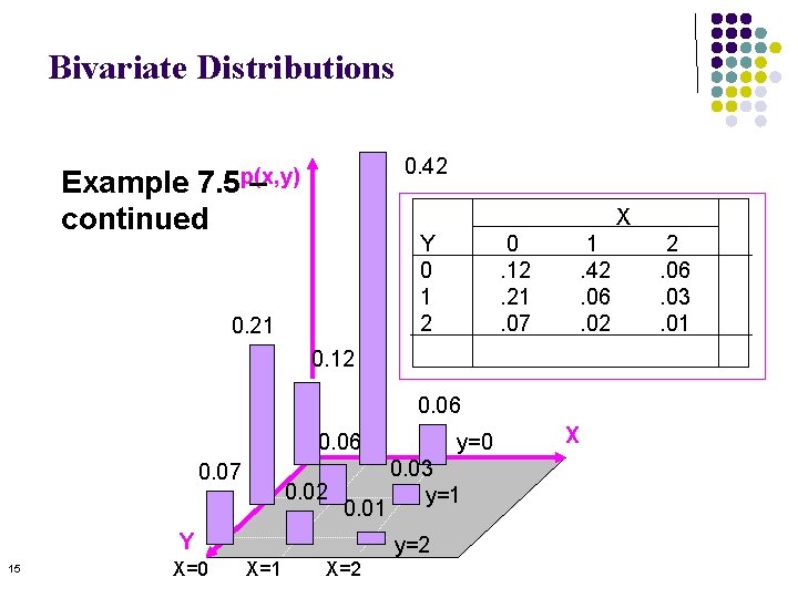
Bivariate Distributions 0. 42 7. 5 p(x, y) – Example continued X Y 0 1 2 0. 21 0. 12. 21. 07 1. 42. 06. 02 0. 12 0. 06 0. 07 0. 02 0. 01 Y 15 X=0 y=0 0. 03 y=1 y=2 X=1 X=2 X 2. 06. 03. 01

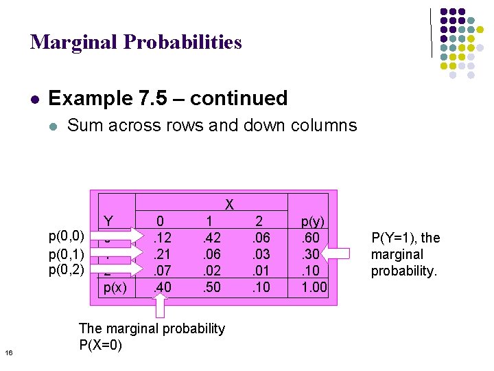
Marginal Probabilities l Example 7. 5 – continued l Sum across rows and down columns X p(0, 0) p(0, 1) p(0, 2) 16 Y 0 1 2 p(x) 0. 12. 21. 07. 40 1. 42. 06. 02. 50 The marginal probability P(X=0) 2. 06. 03. 01. 10 p(y). 60. 30. 10 1. 00 P(Y=1), the marginal probability.

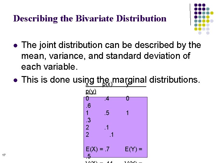
Describing the Bivariate Distribution l l The joint distribution can be described by the mean, variance, and standard deviation of each variable. This is done using the marginal distributions. x p(x) y p(y) 0. 6 1. 3 2 2 17 . 4 0 . 5 1 . 1. 1 E(X) =. 7. 5 E(Y) =

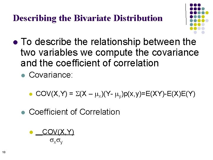
Describing the Bivariate Distribution l To describe the relationship between the two variables we compute the covariance and the coefficient of correlation l Covariance: l l Coefficient of Correlation l 18 COV(X, Y) = S(X – mx)(Y- my)p(x, y)=E(XY)-E(X)E(Y) COV(X, Y) sxsy

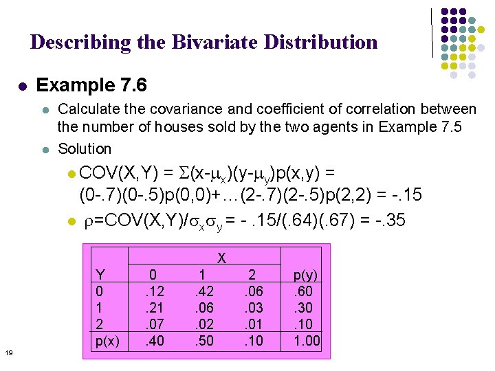
Describing the Bivariate Distribution l Example 7. 6 l l Calculate the covariance and coefficient of correlation between the number of houses sold by the two agents in Example 7. 5 Solution = S(x-mx)(y-my)p(x, y) = (0 -. 7)(0 -. 5)p(0, 0)+…(2 -. 7)(2 -. 5)p(2, 2) = -. 15 l r=COV(X, Y)/sxsy = -. 15/(. 64)(. 67) = -. 35 l COV(X, Y) X Y 0 1 2 p(x) 19 0. 12. 21. 07. 40 1. 42. 06. 02. 50 2. 06. 03. 01. 10 p(y). 60. 30. 10 1. 00

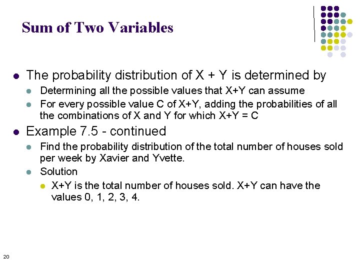
Sum of Two Variables l The probability distribution of X + Y is determined by l l l Example 7. 5 - continued l l 20 Determining all the possible values that X+Y can assume For every possible value C of X+Y, adding the probabilities of all the combinations of X and Y for which X+Y = C Find the probability distribution of the total number of houses sold per week by Xavier and Yvette. Solution l X+Y is the total number of houses sold. X+Y can have the values 0, 1, 2, 3, 4.

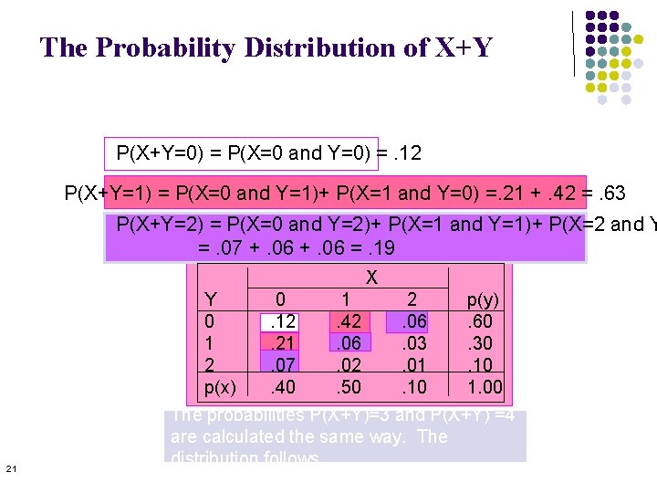
The Probability Distribution of X+Y P(X+Y=0) = P(X=0 and Y=0) =. 12 P(X+Y=1) = P(X=0 and Y=1)+ P(X=1 and Y=0) =. 21 +. 42 =. 63 P(X+Y=2) = P(X=0 and Y=2)+ P(X=1 and Y=1)+ P(X=2 and Y =. 07 +. 06 =. 19 X 21 Y 0 1 2 p(y) 0. 12. 42. 06. 60 1. 21. 06. 03. 30 2. 07. 02. 01. 10 p(x). 40. 50. 10 1. 00 The probabilities P(X+Y)=3 and P(X+Y) =4 are calculated the same way. The distribution follows

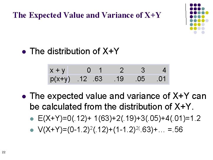
The Expected Value and Variance of X+Y l The distribution of X+Y x+y p(x+y) l 2. 19 3. 05 4. 01 The expected value and variance of X+Y can be calculated from the distribution of X+Y. l l 22 0 1. 12. 63 E(X+Y)=0(. 12)+ 1(63)+2(. 19)+3(. 05)+4(. 01)=1. 2 V(X+Y)=(0 -1. 2)2(. 12)+(1 -1. 2)2(. 63)+… =. 56

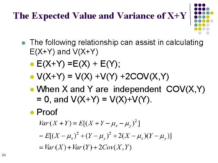
The Expected Value and Variance of X+Y l The following relationship can assist in calculating E(X+Y) and V(X+Y) E(X+Y) =E(X) + E(Y); l V(X+Y) = V(X) +V(Y) +2 COV(X, Y) l When X and Y are independent COV(X, Y) = 0, and V(X+Y) = V(X)+V(Y). l Proof l 23

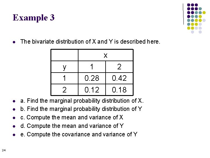
Example 3 l The bivariate distribution of X and Y is described here. x l l l 24 y 1 2 1 0. 28 0. 42 2 0. 18 a. Find the marginal probability distribution of X. b. Find the marginal probability distribution of Y c. Compute the mean and variance of X d. Compute the mean and variance of Y e. Compute the covariance and variance of Y

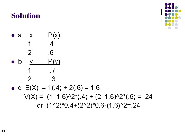
Solution l l l 25 a x P(x) 1. 4 2. 6 b y P(y) 1. 7 2. 3 c E(X) = 1(. 4) + 2(. 6) = 1. 6 V(X) = (1– 1. 6)^2*(. 4) + (2– 1. 6)^2*(. 6) =. 24 or (1^2)*0. 4+(2^2)*0. 6 -(1. 6)^2=. 24

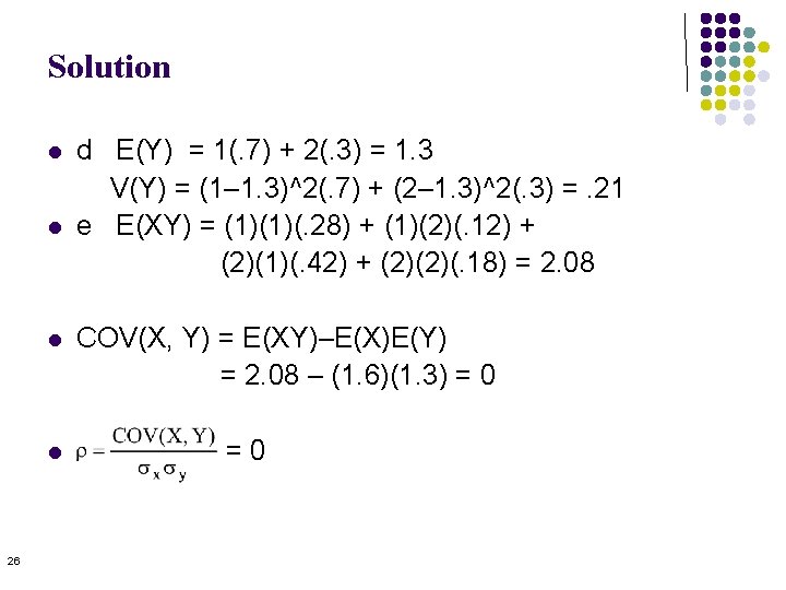
Solution l l 26 d E(Y) = 1(. 7) + 2(. 3) = 1. 3 V(Y) = (1– 1. 3)^2(. 7) + (2– 1. 3)^2(. 3) =. 21 e E(XY) = (1)(1)(. 28) + (1)(2)(. 12) + (2)(1)(. 42) + (2)(2)(. 18) = 2. 08 COV(X, Y) = E(XY)–E(X)E(Y) = 2. 08 – (1. 6)(1. 3) = 0 =0

The Binomial Distribution l l The binomial experiment can result in only one of two possible outcomes. Binomial Experiment l l l Binomial Random Variable l l 27 There are n trials (n is finite and fixed). Each trial can result in a success or a failure. The probability p of success is the same for all the trials. All the trials of the experiment are independent The binomial random variable counts the number of successes in n trials of the binomial experiment. By definition, this is a discrete random variable.

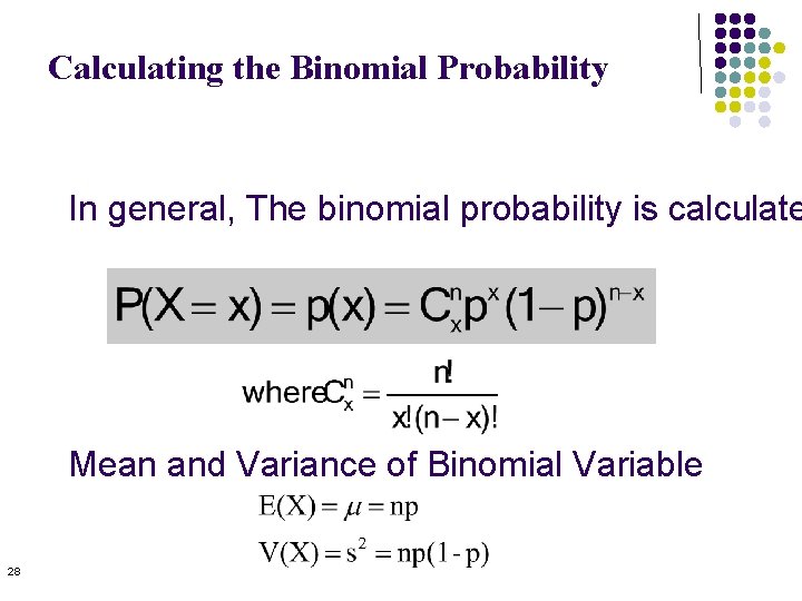
Calculating the Binomial Probability In general, The binomial probability is calculate Mean and Variance of Binomial Variable 28

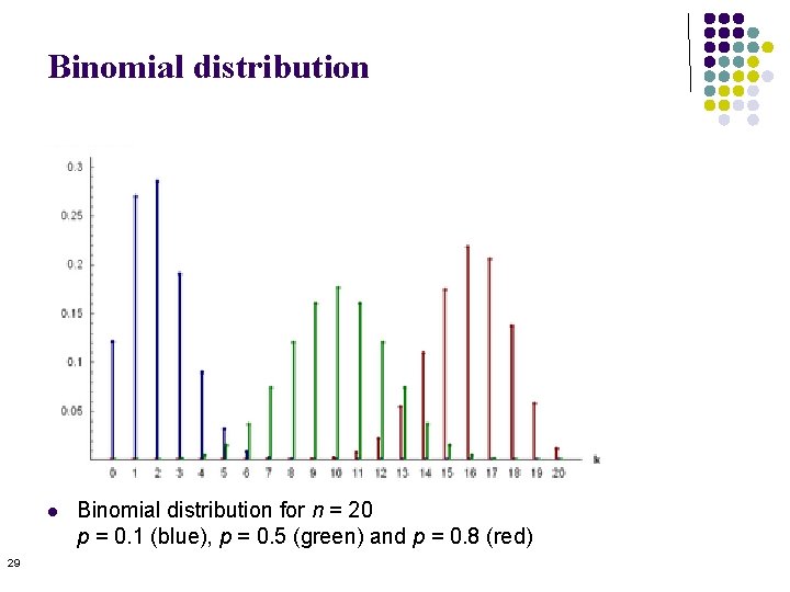
Binomial distribution l 29 Binomial distribution for n = 20 p = 0. 1 (blue), p = 0. 5 (green) and p = 0. 8 (red)

Example 4 l a. b. 30 In the game of blackjack as played in casinos in Las Vegas, Atlantic City, Niagara Falls, as well as many other cities, the dealer has the advantages. Most players do not play very well. As a result, the probability that the average player wins a about 45%. Find the probability that an average player wins twice in 5 hands ten or more times in 25 hands

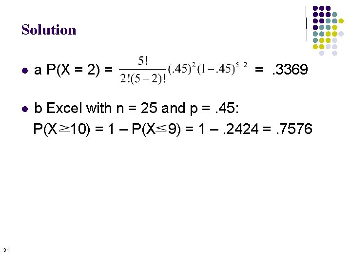
Solution 31 l a P(X = 2) = =. 3369 l b Excel with n = 25 and p =. 45: P(X 10) = 1 – P(X 9) = 1 –. 2424 =. 7576

Poisson Distribution 32 l The Poisson experiment typically fits cases of rare events that occur over a fixed amount of time or within a specified region l Typical cases l The number of errors a typist makes per page l The number of customers entering a service station per hour l The number of telephone calls received by a switchboard per hour.

Properties of the Poisson Experiment l The number of successes (events) that occur in a certain time interval is independent of the number of successes that occur in another time interval. l The probability of a success in a certain time interval is l the same for all time intervals of the same size, l proportional to the length of the interval. The probability that two or more successes will occur in an interval approaches zero as the interval becomes smaller. l 33

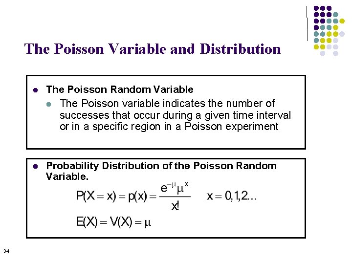
The Poisson Variable and Distribution 34 l The Poisson Random Variable l The Poisson variable indicates the number of successes that occur during a given time interval or in a specific region in a Poisson experiment l Probability Distribution of the Poisson Random Variable.

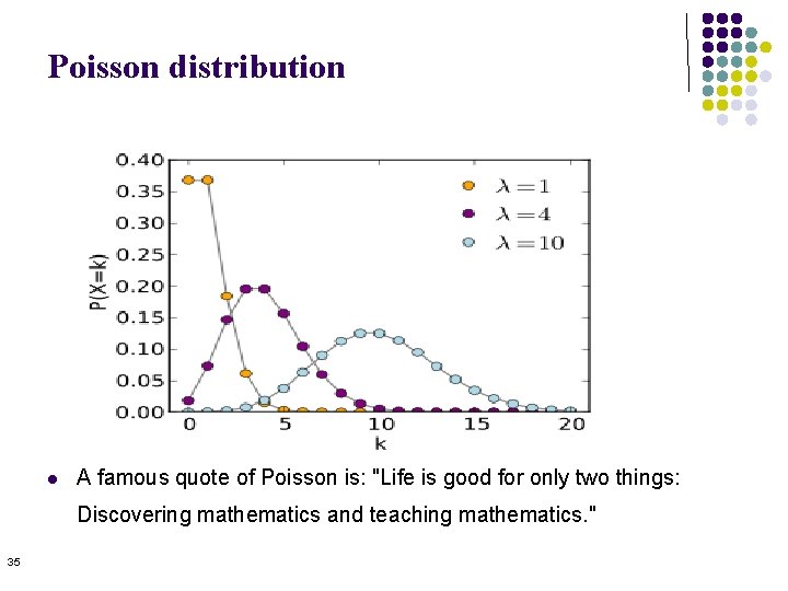
Poisson distribution l A famous quote of Poisson is: "Life is good for only two things: Discovering mathematics and teaching mathematics. " 35

Example 5 l a. b. 36 The number of students who seek assistance with their statistics assignments is Poisson distributed with a mean of three per day. What is the probability that no student seek assistance tomorrow? Find the probability that 10 students seek assistance in a week.

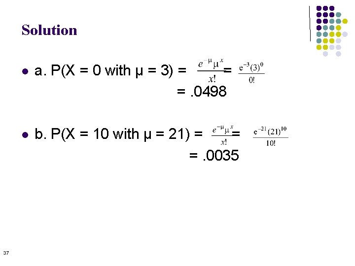
Solution 37 l a. P(X = 0 with μ = 3) = = =. 0498 l b. P(X = 10 with μ = 21) = = =. 0035