Random Variables and Probability Distributions Chapter 4 Never

Random Variables and Probability Distributions Chapter 4 “Never draw to an inside straight. ” from Maxims Learned at My Mother’s Knee MGMT 242 Spring, 1999

Goals for Chapter 4 • Define Random Variable, Probability Distribution • Understand Calculate Expected Value • Understand Calculate Variance, Standard Deviation • Two Random Variables--Understand – Statistical Independence of Two Random Variables – Covariance & Correlation of Two Random Variables • Applications of the Above MGMT 242 Spring, 1999

Random Variables • Refers to possible numerical values that will be the outcome of an experiment or trial and that will vary randomly; • Notation: uppercase letters for last part of alphabet--X, Y, Z • Derived from hypothetical population (infinite number), the members of which will have different values of the random variable • Example--let Y = height of females between 18 and 20 years of age; population is infinite number of females between 18 and 20 • Actual measurements are carried out on a sample, which is randomly chosen from population. MGMT 242 Spring, 1999

Probability Distributions • A probability distribution gives the probability for a specific value of the random variable: – P(Y= y) gives the probability distribution when values for P are specified for specific values of y – example: tossed a coin twice(fair coin); Y is the number of heads that are tossed; possible events: TT, TH, HT, HH; each event is equally probable if coin is a fair coin, so probability of Y=0 (event: TT) is 1/4; probability of Y =2 is 1/4; probability of Y = 1 is 1/4 +1/4 = 1/2; – Thus, for example: • P(Y=0) = 1/4 • P(Y=1) = 1/2 • P(Y=2) = 1/4 MGMT 242 Spring, 1999

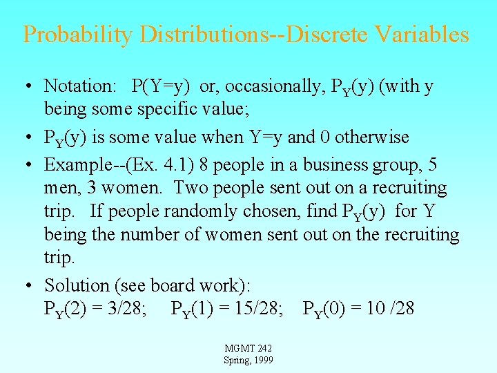
Probability Distributions--Discrete Variables • Notation: P(Y=y) or, occasionally, PY(y) (with y being some specific value; • PY(y) is some value when Y=y and 0 otherwise • Example--(Ex. 4. 1) 8 people in a business group, 5 men, 3 women. Two people sent out on a recruiting trip. If people randomly chosen, find PY(y) for Y being the number of women sent out on the recruiting trip. • Solution (see board work): PY(2) = 3/28; PY(1) = 15/28; PY(0) = 10 /28 MGMT 242 Spring, 1999

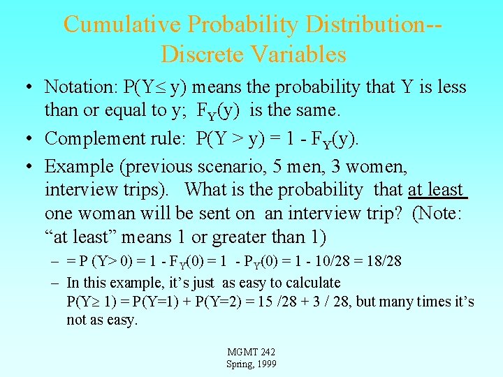
Cumulative Probability Distribution-Discrete Variables • Notation: P(Y y) means the probability that Y is less than or equal to y; FY(y) is the same. • Complement rule: P(Y > y) = 1 - FY(y). • Example (previous scenario, 5 men, 3 women, interview trips). What is the probability that at least one woman will be sent on an interview trip? (Note: “at least” means 1 or greater than 1) – = P (Y> 0) = 1 - FY(0) = 1 - PY(0) = 1 - 10/28 = 18/28 – In this example, it’s just as easy to calculate P(Y 1) = P(Y=1) + P(Y=2) = 15 /28 + 3 / 28, but many times it’s not as easy. MGMT 242 Spring, 1999

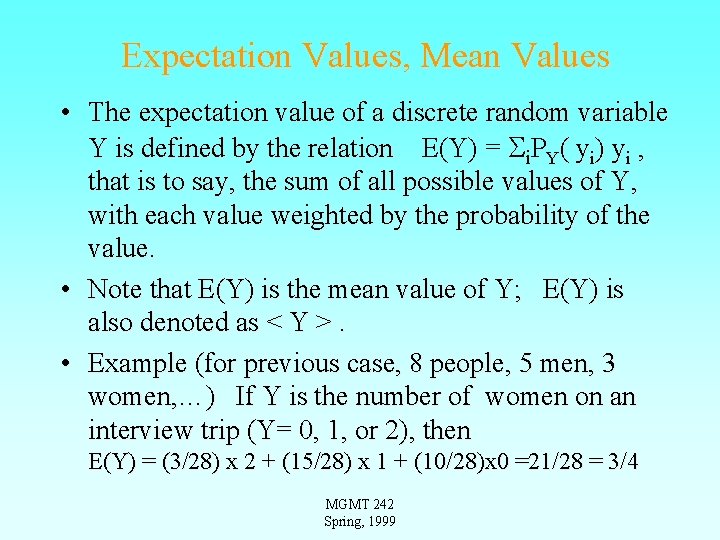
Expectation Values, Mean Values • The expectation value of a discrete random variable Y is defined by the relation E(Y) = i. PY( yi) yi , that is to say, the sum of all possible values of Y, with each value weighted by the probability of the value. • Note that E(Y) is the mean value of Y; E(Y) is also denoted as < Y >. • Example (for previous case, 8 people, 5 men, 3 women, …) If Y is the number of women on an interview trip (Y= 0, 1, or 2), then E(Y) = (3/28) x 2 + (15/28) x 1 + (10/28)x 0 =21/28 = 3/4 MGMT 242 Spring, 1999

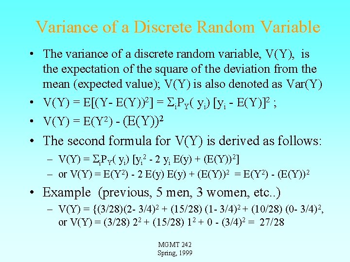
Variance of a Discrete Random Variable • The variance of a discrete random variable, V(Y), is the expectation of the square of the deviation from the mean (expected value); V(Y) is also denoted as Var(Y) • V(Y) = E[(Y- E(Y))2] = i. PY( yi) [yi - E(Y)]2 ; • V(Y) = E(Y 2) - (E(Y))2 • The second formula for V(Y) is derived as follows: – V(Y) = i. PY( yi) [yi 2 - 2 yi E(y) + (E(Y))2] – or V(Y) = E(Y 2) - 2 E(y) + (E(Y))2 = E(Y 2) - (E(Y))2 • Example (previous, 5 men, 3 women, etc. . ) – V(Y) = {(3/28)(2 - 3/4)2 + (15/28) (1 - 3/4)2 + (10/28) (0 - 3/4)2, or V(Y) = (3/28) 22 + (15/28) 12 + 0 - (3/4)2 = 27/28 MGMT 242 Spring, 1999

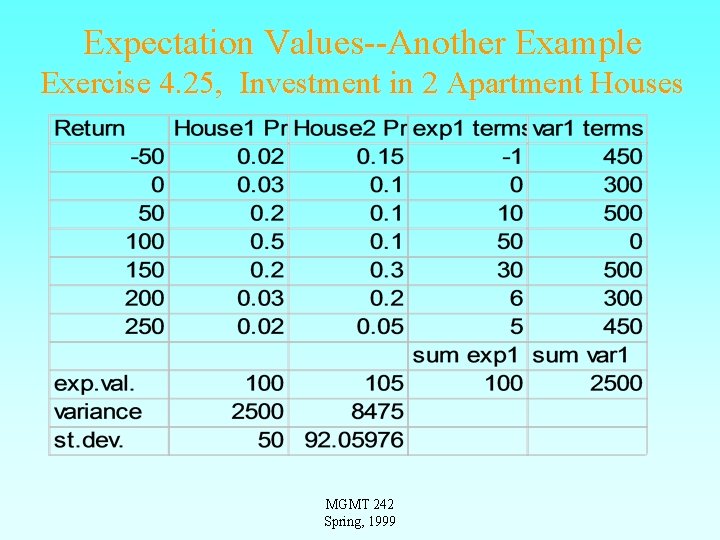
Expectation Values--Another Example Exercise 4. 25, Investment in 2 Apartment Houses MGMT 242 Spring, 1999

Continuous Random Variables • Reasons for using a continuous variable rather than discrete – Many, many values (e. g. salaries)--too many to take as discrete; – Model for probability distribution makes it convenient or necessary to use a continuous variable- • Uniform Distribution (any value between set limits equally likely) • Exponential Distribution (waiting times, delay times) • Normal (Gaussian) Distribution, the “Bell Shaped Curve” (many measurement values follow a normal distribution either directly or after an appropriate transformation of variables; also mean values of samples follow a normal distribution, generally. ) MGMT 242 Spring, 1999

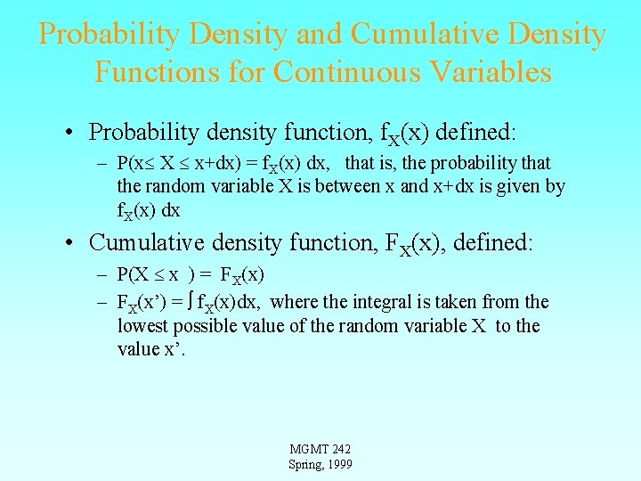
Probability Density and Cumulative Density Functions for Continuous Variables • Probability density function, f. X(x) defined: – P(x X x+dx) = f. X(x) dx, that is, the probability that the random variable X is between x and x+dx is given by f. X(x) dx • Cumulative density function, FX(x), defined: – P(X x ) = FX(x) – FX(x’) = f. X(x)dx, where the integral is taken from the lowest possible value of the random variable X to the value x’. MGMT 242 Spring, 1999

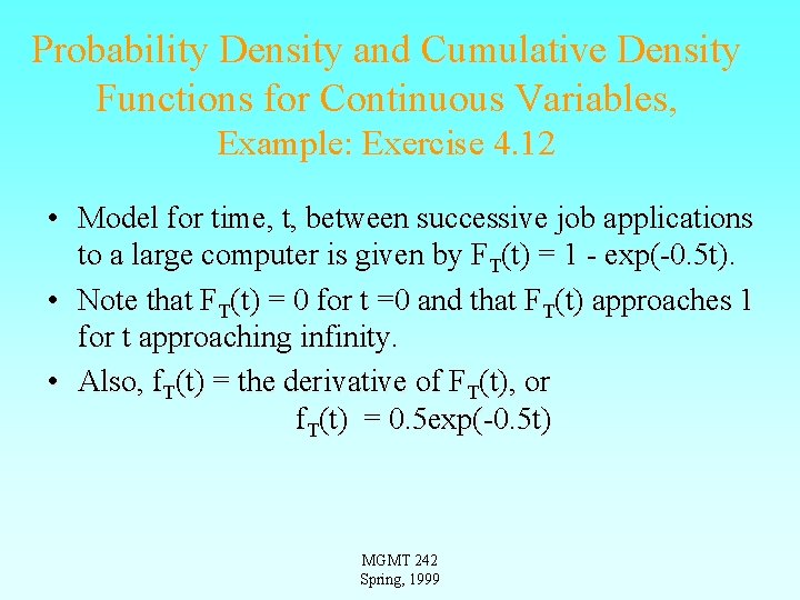
Probability Density and Cumulative Density Functions for Continuous Variables, Example: Exercise 4. 12 • Model for time, t, between successive job applications to a large computer is given by FT(t) = 1 - exp(-0. 5 t). • Note that FT(t) = 0 for t =0 and that FT(t) approaches 1 for t approaching infinity. • Also, f. T(t) = the derivative of FT(t), or f. T(t) = 0. 5 exp(-0. 5 t) MGMT 242 Spring, 1999

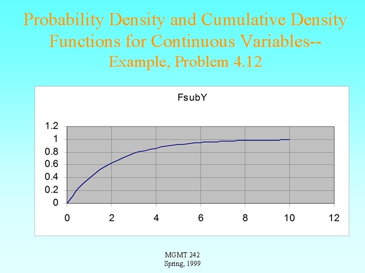
Probability Density and Cumulative Density Functions for Continuous Variables-Example, Problem 4. 12 MGMT 242 Spring, 1999

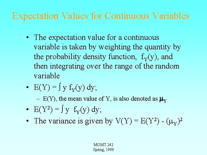
Expectation Values for Continuous Variables • The expectation value for a continuous variable is taken by weighting the quantity by the probability density function, f. Y(y), and then integrating over the range of the random variable • E(Y) = y f. Y(y) dy; – E(Y), the mean value of Y, is also denoted as Y • E(Y 2) = y f. Y(y) dy; • The variance is given by V(Y) = E(Y 2) - ( Y)2 MGMT 242 Spring, 1999

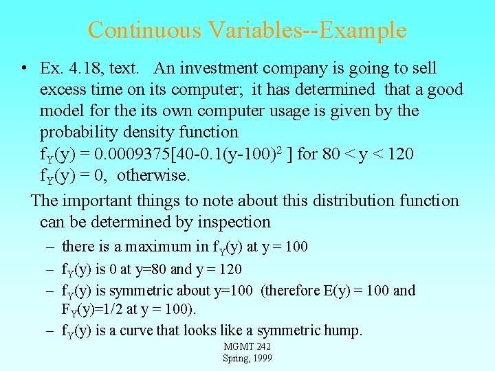
Continuous Variables--Example • Ex. 4. 18, text. An investment company is going to sell excess time on its computer; it has determined that a good model for the its own computer usage is given by the probability density function f. Y(y) = 0. 0009375[40 -0. 1(y-100)2 ] for 80 < y < 120 f. Y(y) = 0, otherwise. The important things to note about this distribution function can be determined by inspection – there is a maximum in f. Y(y) at y = 100 – f. Y(y) is 0 at y=80 and y = 120 – f. Y(y) is symmetric about y=100 (therefore E(y) = 100 and FY(y)=1/2 at y = 100). – f. Y(y) is a curve that looks like a symmetric hump. MGMT 242 Spring, 1999

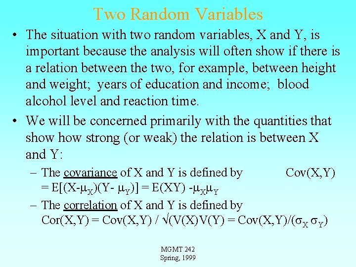
Two Random Variables • The situation with two random variables, X and Y, is important because the analysis will often show if there is a relation between the two, for example, between height and weight; years of education and income; blood alcohol level and reaction time. • We will be concerned primarily with the quantities that show strong (or weak) the relation is between X and Y: – The covariance of X and Y is defined by Cov(X, Y) = E[(X- X)(Y- Y)] = E(XY) - X Y – The correlation of X and Y is defined by Cor(X, Y) = Cov(X, Y) / (V(X)V(Y) = Cov(X, Y)/( X Y) MGMT 242 Spring, 1999

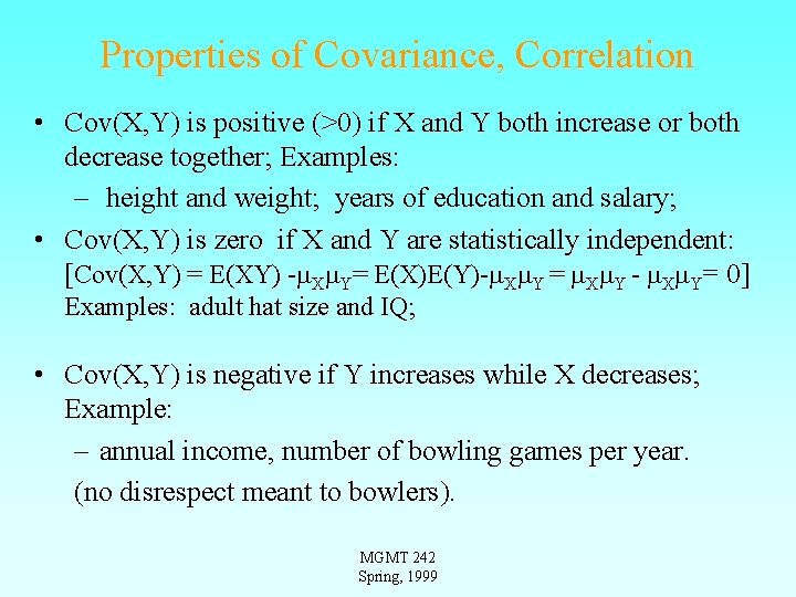
Properties of Covariance, Correlation • Cov(X, Y) is positive (>0) if X and Y both increase or both decrease together; Examples: – height and weight; years of education and salary; • Cov(X, Y) is zero if X and Y are statistically independent: [Cov(X, Y) = E(XY) - X Y= E(X)E(Y)- X Y = X Y - X Y= 0] Examples: adult hat size and IQ; • Cov(X, Y) is negative if Y increases while X decreases; Example: – annual income, number of bowling games per year. (no disrespect meant to bowlers). MGMT 242 Spring, 1999

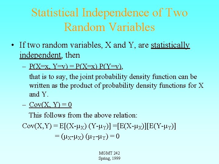
Statistical Independence of Two Random Variables • If two random variables, X and Y, are statistically independent, then – P(X=x, Y=y) = P(X=x) P(Y=y), that is to say, the joint probability density function can be written as the product of probability density functions for X and Y. – Cov(X, Y) = 0 This follows from the above relation: Cov(X, Y) = E[(X-µX) (Y-µY)] =[E(X-µX)][E(Y-µY)] = (µX-µX) (µY-µY) = 0 MGMT 242 Spring, 1999