Random Swap algorithm Pasi Frnti 24 4 2018

Random Swap algorithm Pasi Fränti 24. 4. 2018

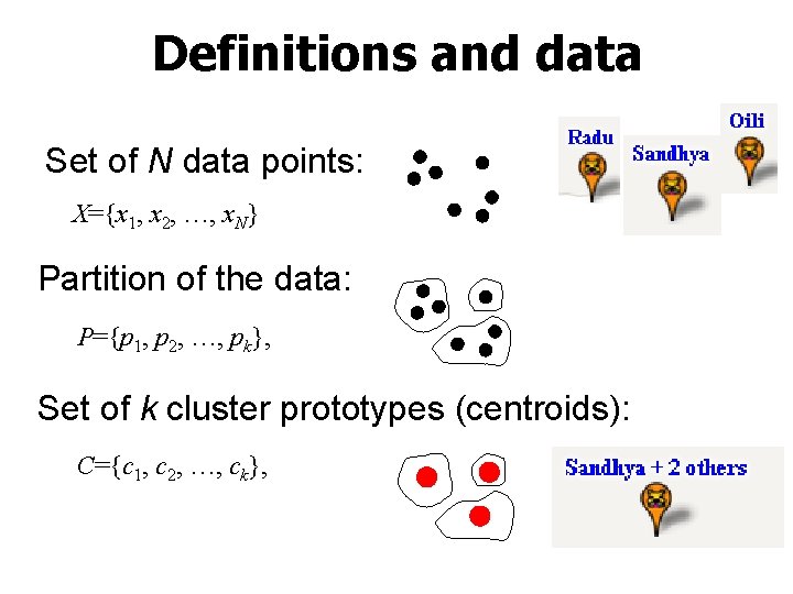
Definitions and data Set of N data points: X={x 1, x 2, …, x. N} Partition of the data: P={p 1, p 2, …, pk}, Set of k cluster prototypes (centroids): C={c 1, c 2, …, ck},

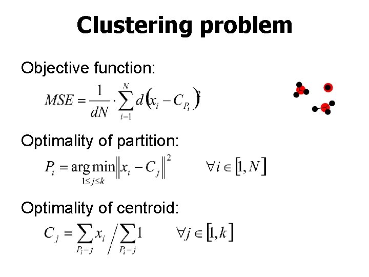
Clustering problem Objective function: Optimality of partition: Optimality of centroid:

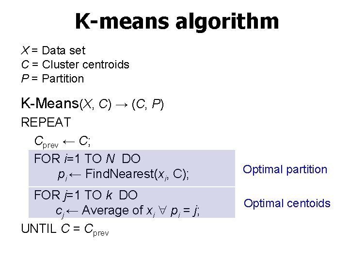
K-means algorithm X = Data set C = Cluster centroids P = Partition K-Means(X, C) → (C, P) REPEAT Cprev ← C; FOR i=1 TO N DO pi ← Find. Nearest(xi, C); FOR j=1 TO k DO cj ← Average of xi pi = j; UNTIL C = Cprev Optimal partition Optimal centoids

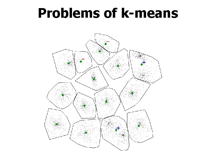
Problems of k-means

Swapping strategy

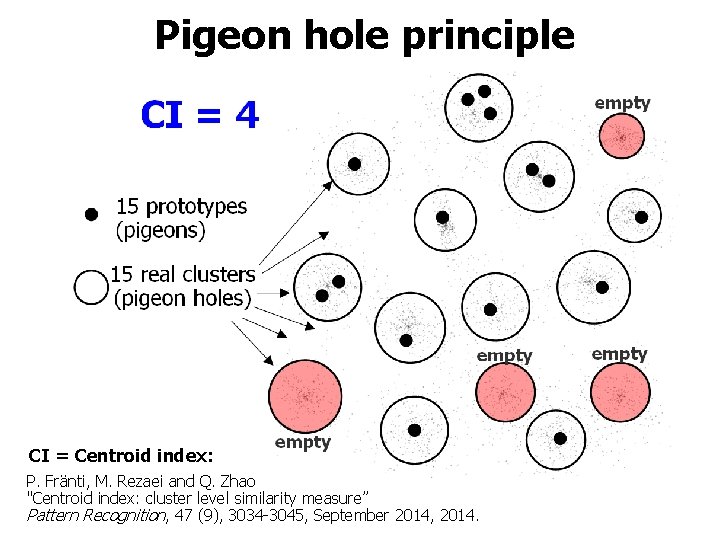
Pigeon hole principle CI = Centroid index: P. Fränti, M. Rezaei and Q. Zhao "Centroid index: cluster level similarity measure” Pattern Recognition, 47 (9), 3034 -3045, September 2014, 2014.

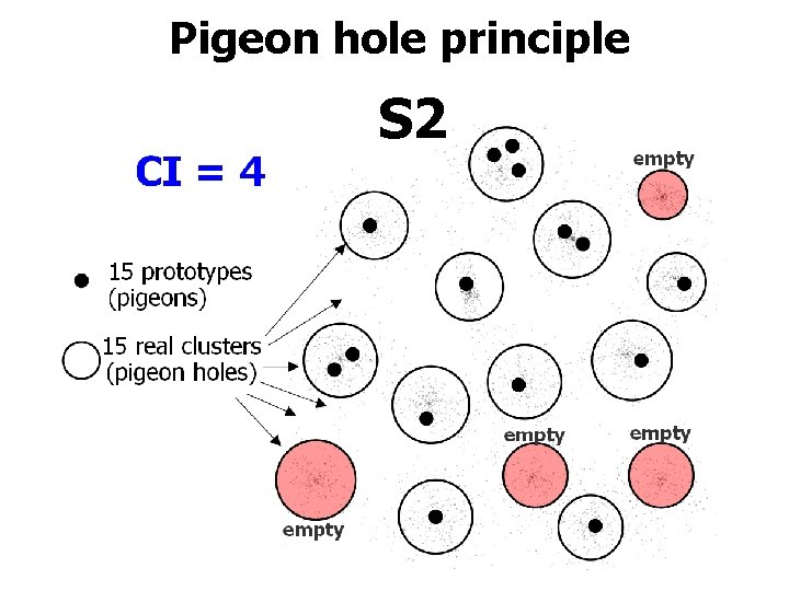
Pigeon hole principle S 2

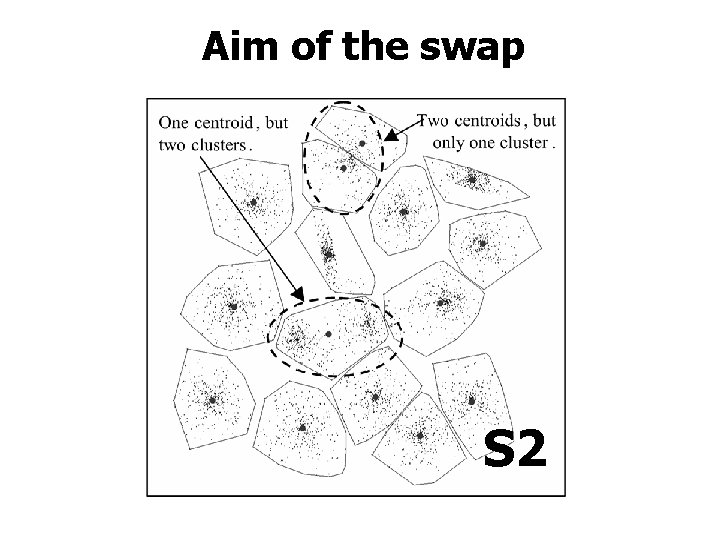
Aim of the swap S 2

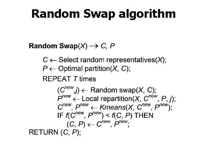
Random Swap algorithm

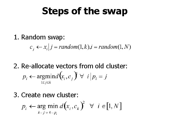
Steps of the swap 1. Random swap: 2. Re-allocate vectors from old cluster: 3. Create new cluster:

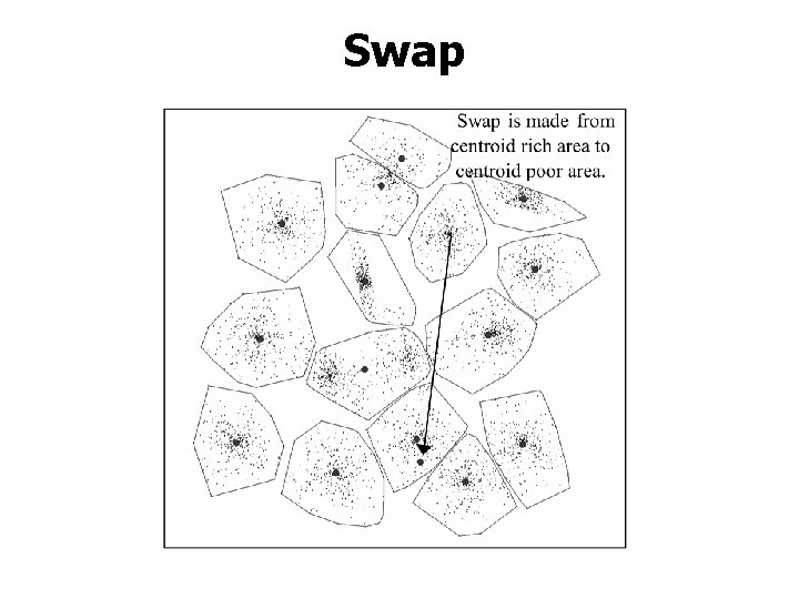
Swap

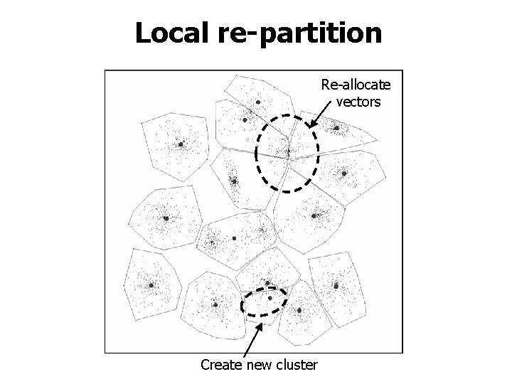
Local re-partition Re-allocate vectors Create new cluster

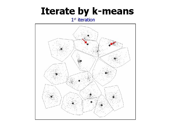
Iterate by k-means 1 st iteration

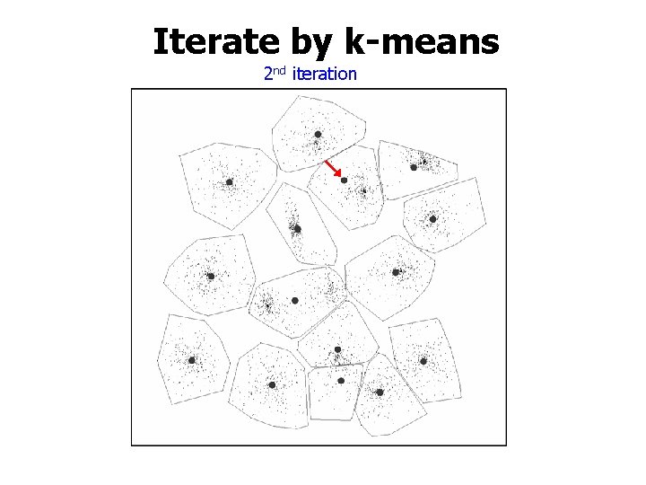
Iterate by k-means 2 nd iteration

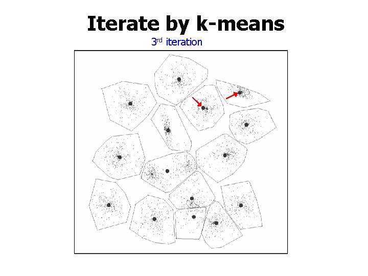
Iterate by k-means 3 rd iteration

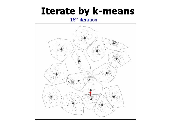
Iterate by k-means 16 th iteration

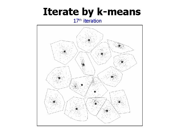
Iterate by k-means 17 th iteration

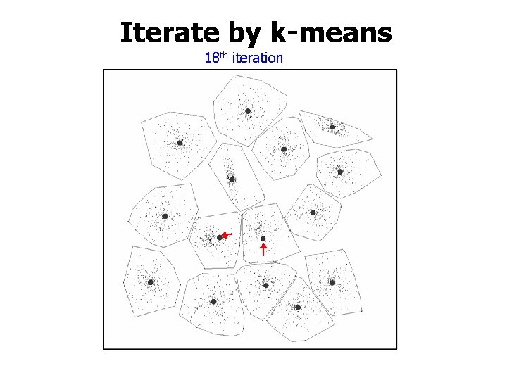
Iterate by k-means 18 th iteration

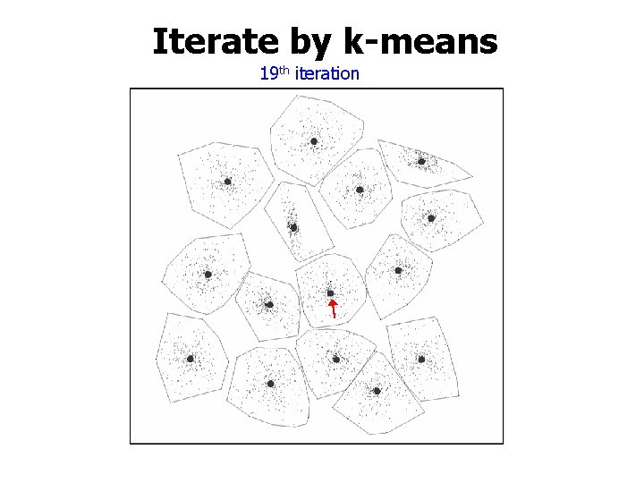
Iterate by k-means 19 th iteration

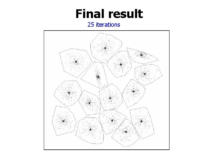
Final result 25 iterations

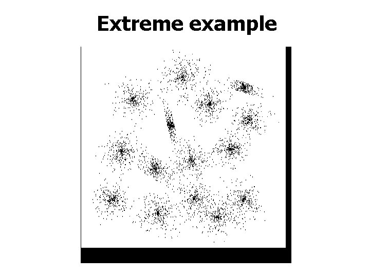
Extreme example

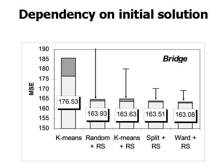
Dependency on initial solution

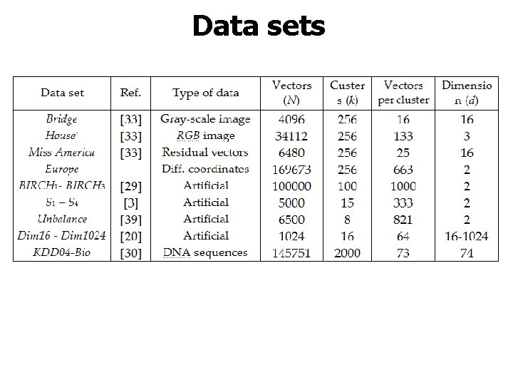
Data sets

Data sets

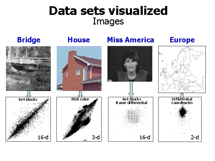
Data sets visualized Images Bridge House RGB color 4 x 4 blocks 16 -d 3 -d Miss America Europe 4 x 4 blocks frame differential Differential coordinates 16 -d 2 -d

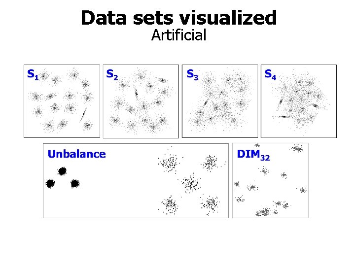
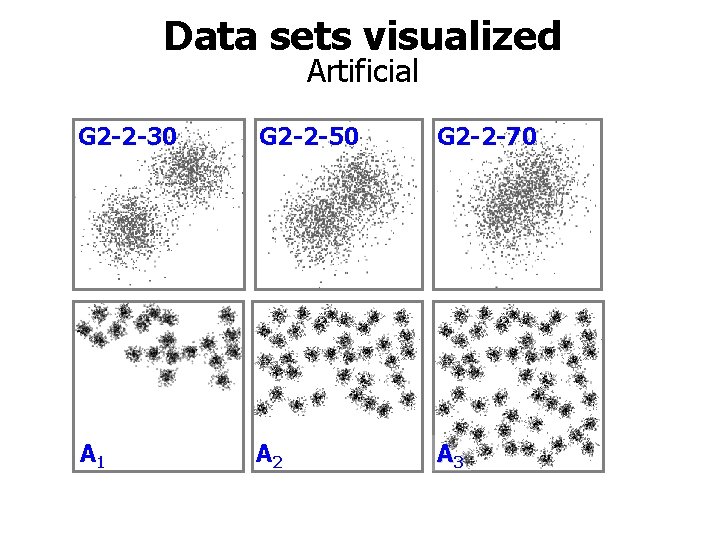
Data sets visualized Artificial

Data sets visualized Artificial G 2 -2 -30 G 2 -2 -50 G 2 -2 -70 A 1 A 2 A 3

Time complexity

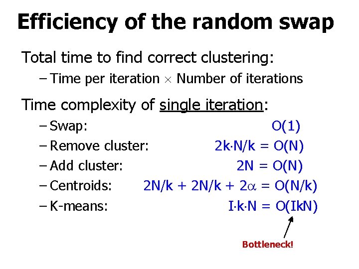
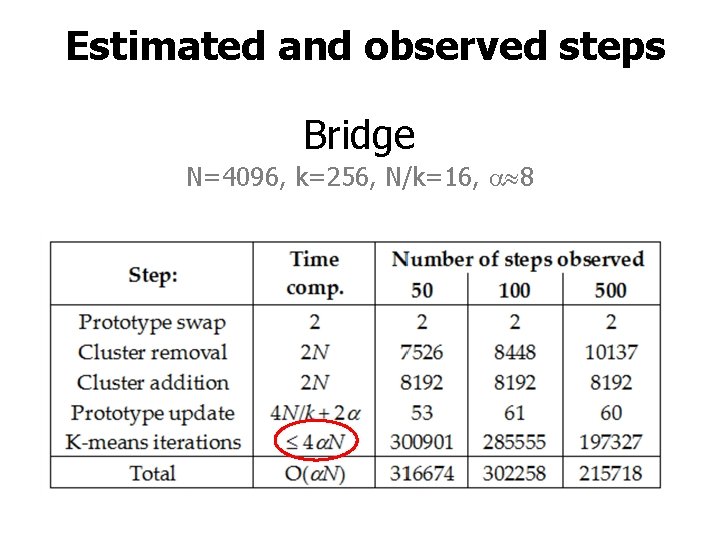
Efficiency of the random swap Total time to find correct clustering: – Time per iteration Number of iterations Time complexity of single iteration: – Swap: O(1) – Remove cluster: 2 k N/k = O(N) – Add cluster: 2 N = O(N) – Centroids: 2 N/k + 2 = O(N/k) – K-means: I k N = O(Ik. N) Bottleneck!

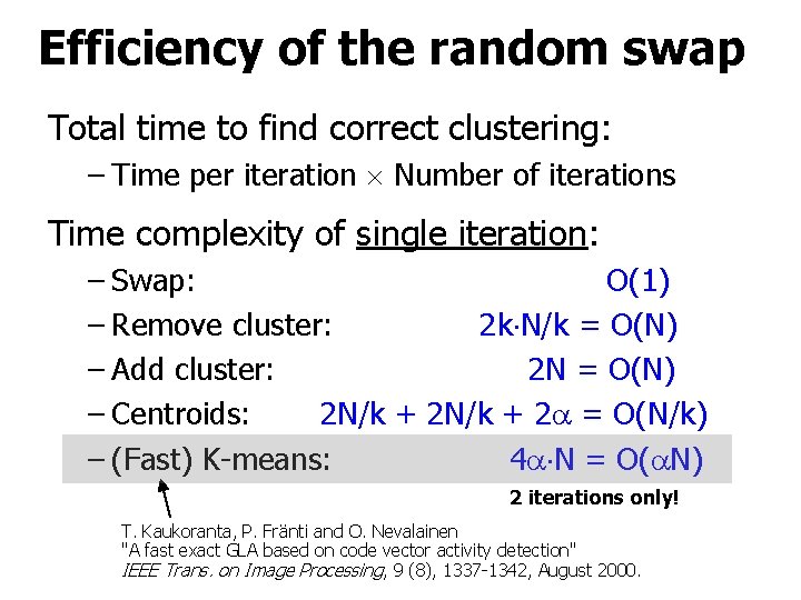
Efficiency of the random swap Total time to find correct clustering: – Time per iteration Number of iterations Time complexity of single iteration: – Swap: O(1) – Remove cluster: 2 k N/k = O(N) – Add cluster: 2 N = O(N) – Centroids: 2 N/k + 2 = O(N/k) – (Fast) K-means: 4 N = O( N) 2 iterations only! T. Kaukoranta, P. Fränti and O. Nevalainen "A fast exact GLA based on code vector activity detection" IEEE Trans. on Image Processing, 9 (8), 1337 -1342, August 2000.

Estimated and observed steps Bridge N=4096, k=256, N/k=16, 8

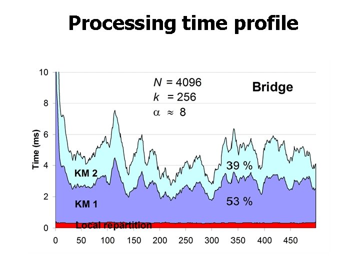
Processing time profile

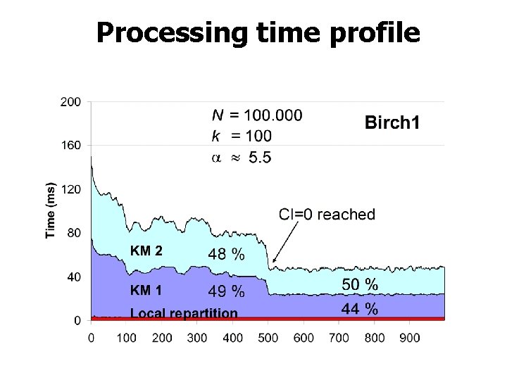
Processing time profile

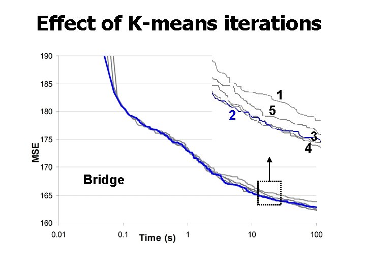
Effect of K-means iterations 2 1 5 3 4 Bridge

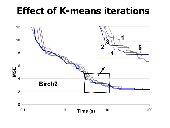
Effect of K-means iterations 2 Birch 2 1 3 4 5

How many swaps?

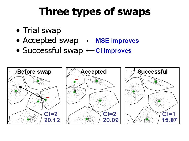
Three types of swaps • Trial swap • Accepted swap • Successful swap Before swap CI=2 20. 12 MSE improves CI improves Accepted CI=2 20. 09 Successful CI=1 15. 87

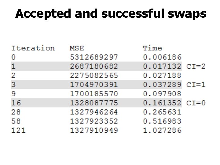
Accepted and successful swaps

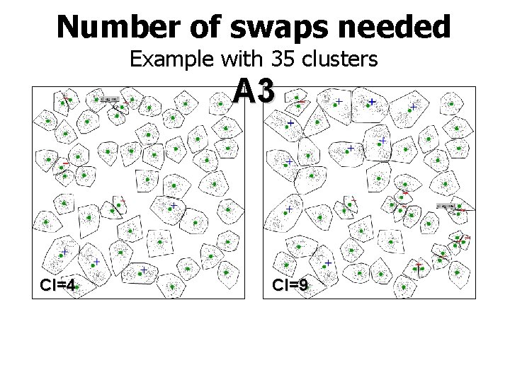
Number of swaps needed Example with 35 clusters A 3 CI=4 CI=9

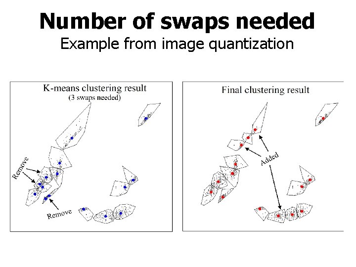
Number of swaps needed Example from image quantization

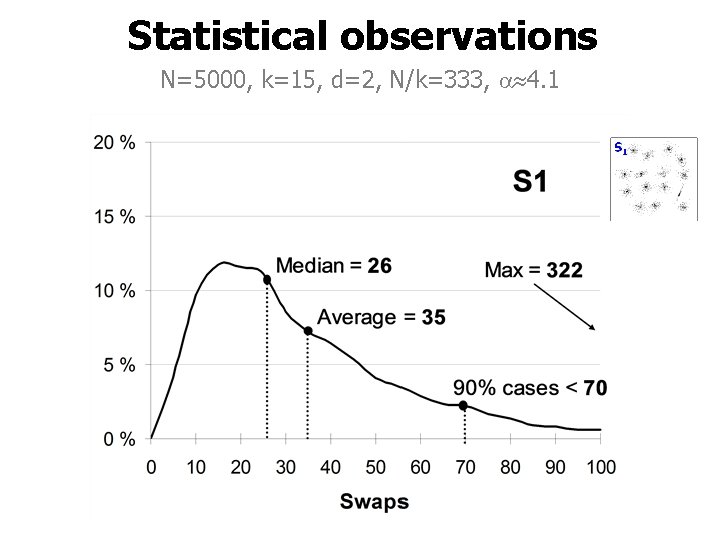
Statistical observations N=5000, k=15, d=2, N/k=333, 4. 1

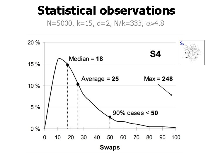
Statistical observations N=5000, k=15, d=2, N/k=333, 4. 8

Theoretical estimation

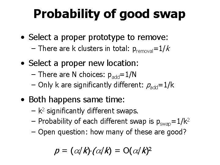
Probability of good swap • Select a proper prototype to remove: – There are k clusters in total: premoval=1/k • Select a proper new location: – There are N choices: padd=1/N – Only k are significantly different: padd=1/k • Both happens same time: – k 2 significantly different swaps. – Probability of each different swap is pswap=1/k 2 – Open question: how many of these are good? p = ( /k) = O( /k)2

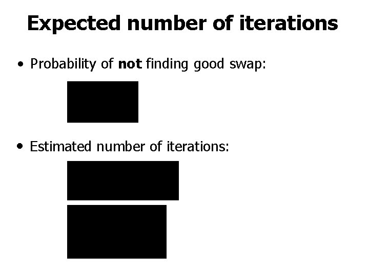
Expected number of iterations • Probability of not finding good swap: • Estimated number of iterations:

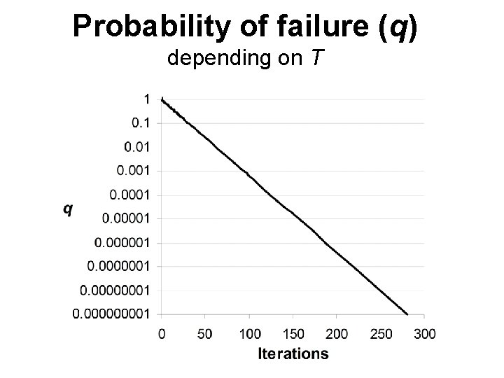
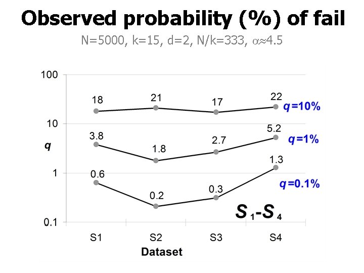
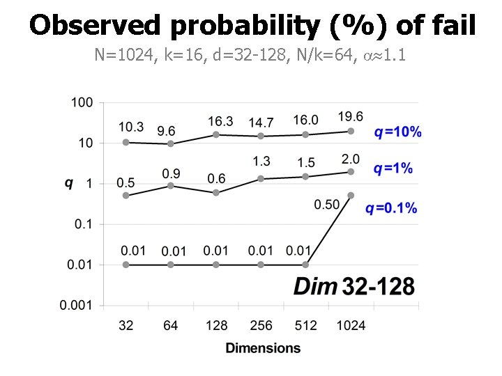
Probability of failure (q) depending on T

Observed probability (%) of fail N=5000, k=15, d=2, N/k=333, 4. 5

Observed probability (%) of fail N=1024, k=16, d=32 -128, N/k=64, 1. 1

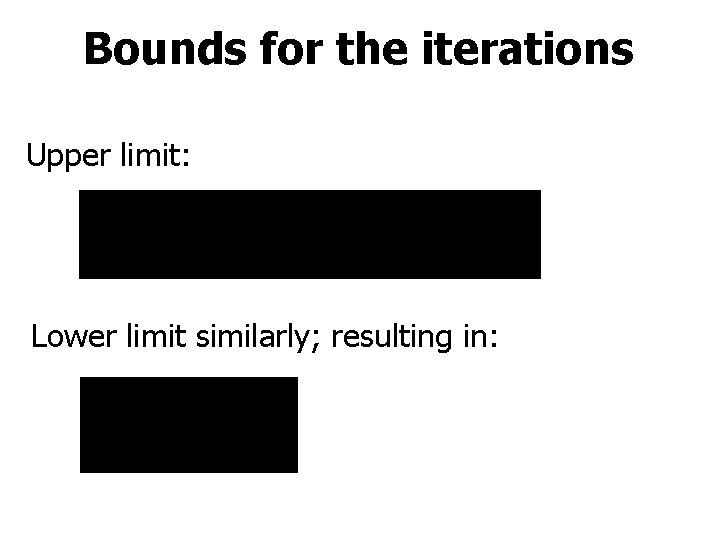
Bounds for the iterations Upper limit: Lower limit similarly; resulting in:

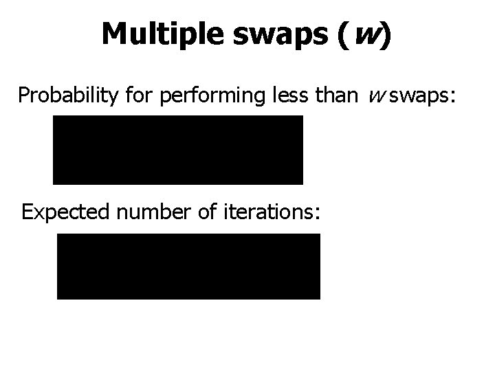
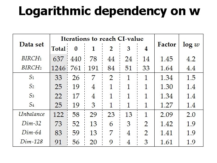
Multiple swaps (w) Probability for performing less than w swaps: Expected number of iterations:

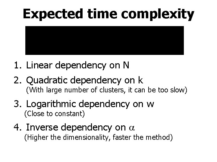
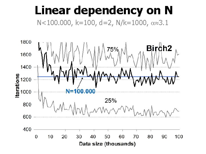
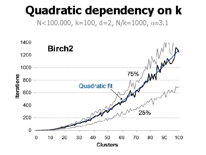
Expected time complexity 1. Linear dependency on N 2. Quadratic dependency on k (With large number of clusters, it can be too slow) 3. Logarithmic dependency on w (Close to constant) 4. Inverse dependency on (Higher the dimensionality, faster the method)

Linear dependency on N N<100. 000, k=100, d=2, N/k=1000, 3. 1

Quadratic dependency on k N<100. 000, k=100, d=2, N/k=1000, 3. 1

Logarithmic dependency on w

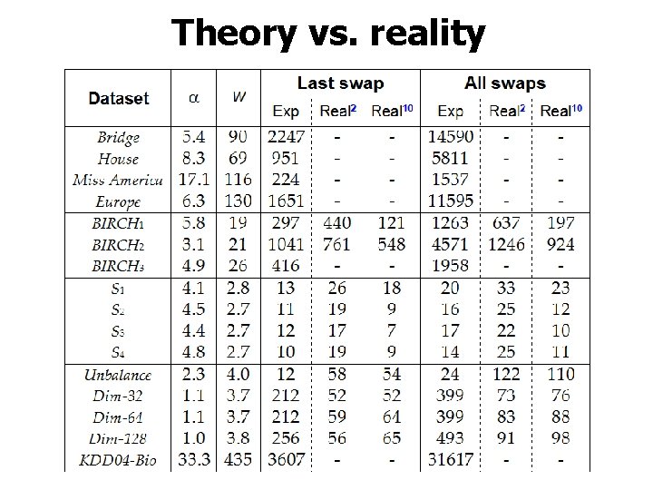
Theory vs. reality

Neighborhood size

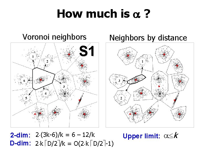
How much is ? Voronoi neighbors Neighbors by distance S 1 2 -dim: 2 (3 k-6)/k = 6 – 12/k D-dim: 2 k D/2 /k = O(2 k D/2 -1) Upper limit: k

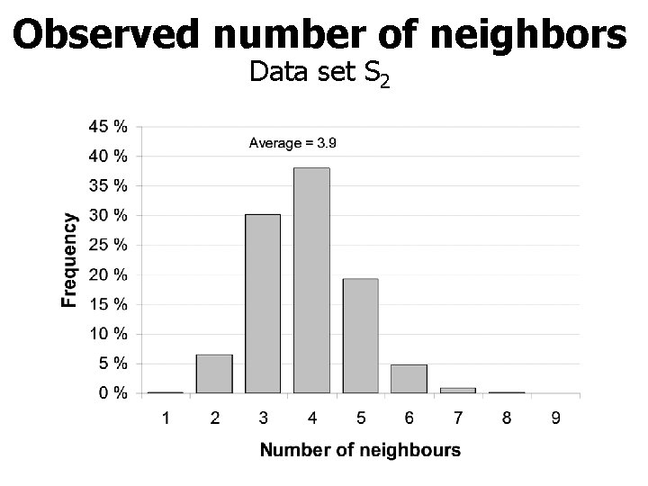
Observed number of neighbors Data set S 2

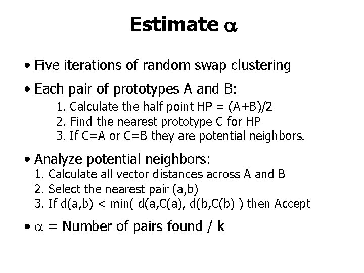
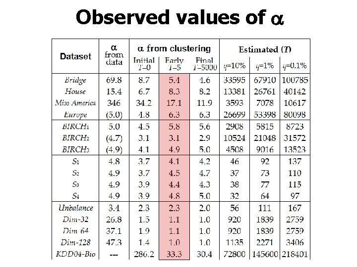
Estimate • Five iterations of random swap clustering • Each pair of prototypes A and B: 1. Calculate the half point HP = (A+B)/2 2. Find the nearest prototype C for HP 3. If C=A or C=B they are potential neighbors. • Analyze potential neighbors: 1. Calculate all vector distances across A and B 2. Select the nearest pair (a, b) 3. If d(a, b) < min( d(a, C(a), d(b, C(b) ) then Accept • = Number of pairs found / k

Observed values of

Optimality

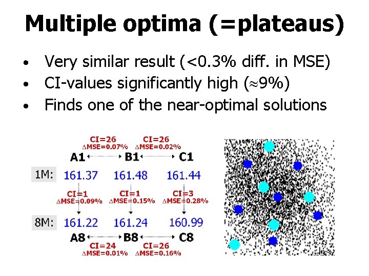
Multiple optima (=plateaus) Very similar result (<0. 3% diff. in MSE) • CI-values significantly high ( 9%) • Finds one of the near-optimal solutions •

Experiments

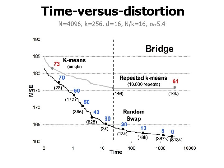
Time-versus-distortion N=4096, k=256, d=16, N/k=16, 5. 4

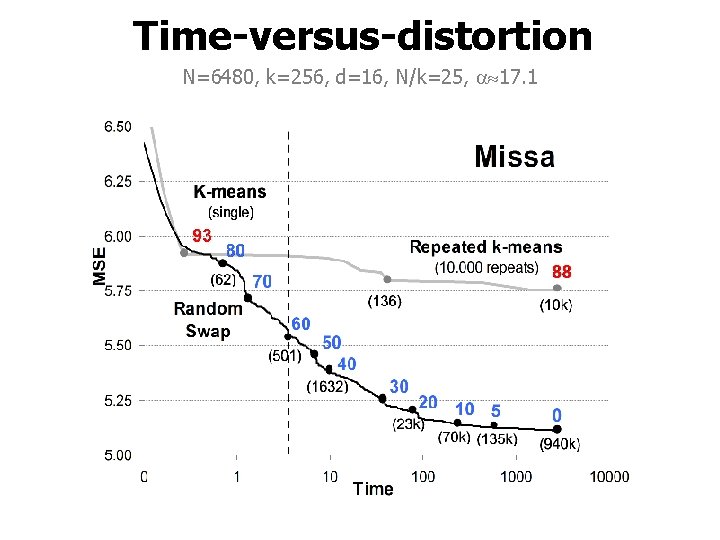
Time-versus-distortion N=6480, k=256, d=16, N/k=25, 17. 1

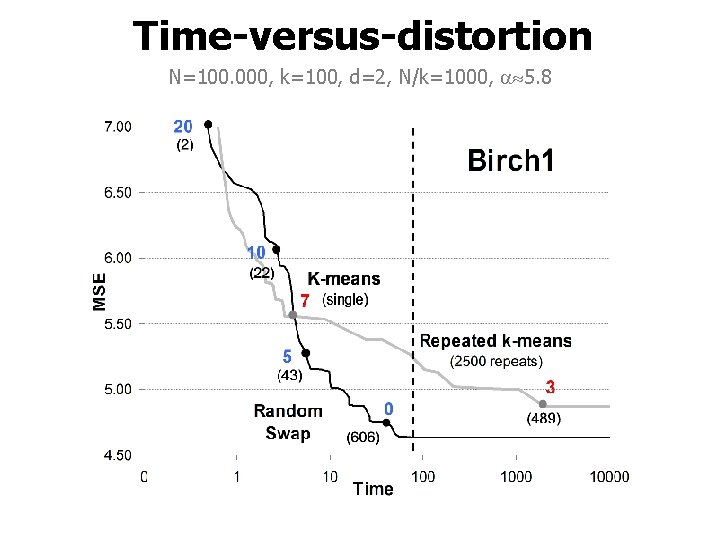
Time-versus-distortion N=100. 000, k=100, d=2, N/k=1000, 5. 8

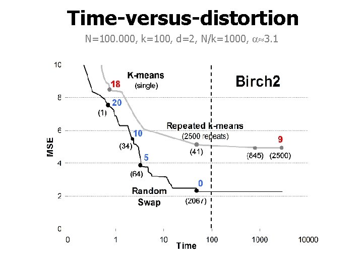
Time-versus-distortion N=100. 000, k=100, d=2, N/k=1000, 3. 1

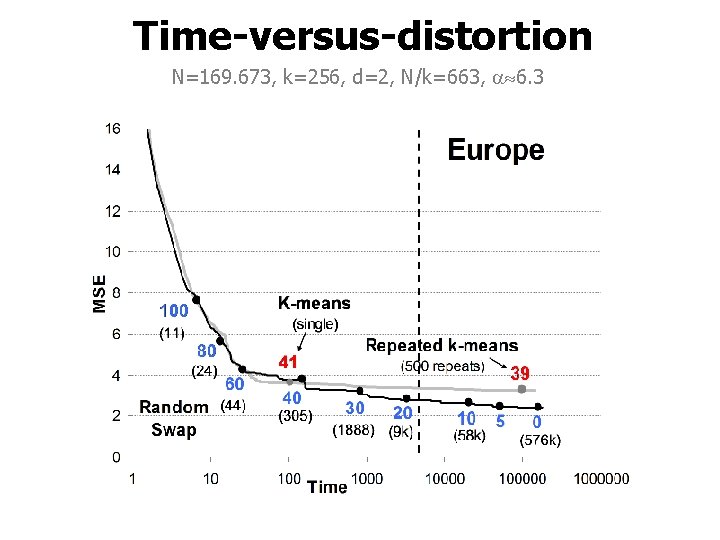
Time-versus-distortion N=169. 673, k=256, d=2, N/k=663, 6. 3

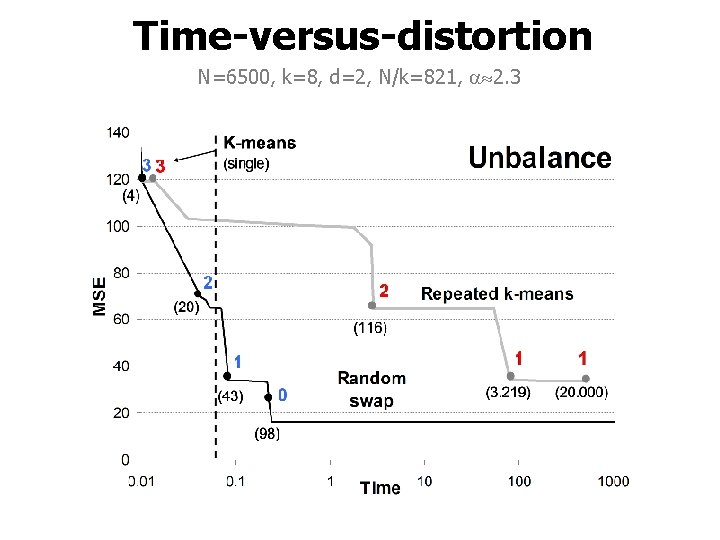
Time-versus-distortion N=6500, k=8, d=2, N/k=821, 2. 3

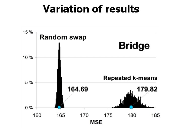
Variation of results

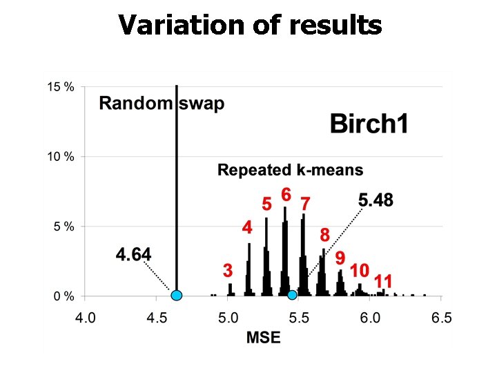
Variation of results

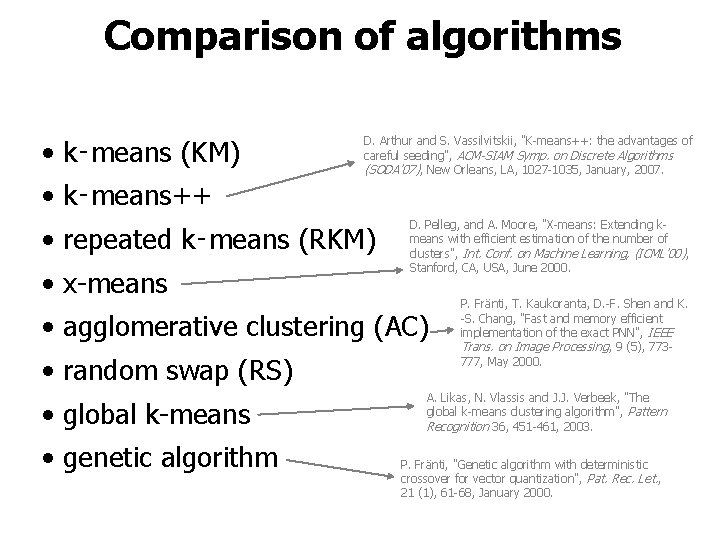
Comparison of algorithms • k‑means (KM) D. Arthur and S. Vassilvitskii, "K-means++: the advantages of careful seeding", ACM-SIAM Symp. on Discrete Algorithms (SODA’ 07), New Orleans, LA, 1027 -1035, January, 2007. • k‑means++ • repeated k‑means (RKM) • x-means D. Pelleg, and A. Moore, "X-means: Extending kmeans with efficient estimation of the number of clusters", Int. Conf. on Machine Learning, (ICML’ 00) , Stanford, CA, USA, June 2000. • agglomerative clustering (AC) • random swap (RS) • global k-means • genetic algorithm P. Fränti, T. Kaukoranta, D. -F. Shen and K. -S. Chang, "Fast and memory efficient implementation of the exact PNN", IEEE Trans. on Image Processing , 9 (5), 773777, May 2000. A. Likas, N. Vlassis and J. J. Verbeek, "The global k-means clustering algorithm", Pattern Recognition 36, 451 -461, 2003. P. Fränti, "Genetic algorithm with deterministic crossover for vector quantization", Pat. Rec. Let. , 21 (1), 61 -68, January 2000.

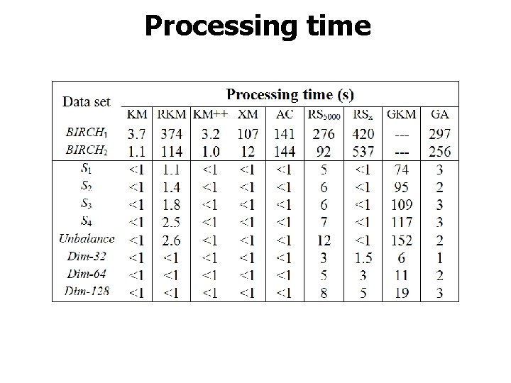
Processing time

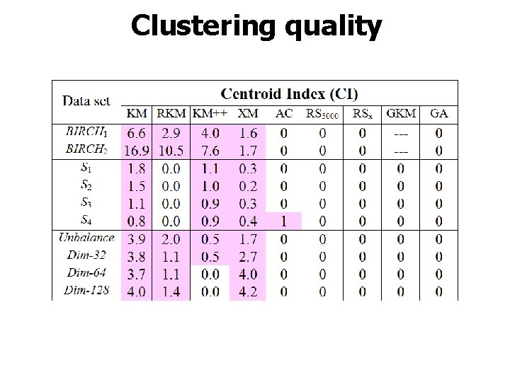
Clustering quality

Conclusions

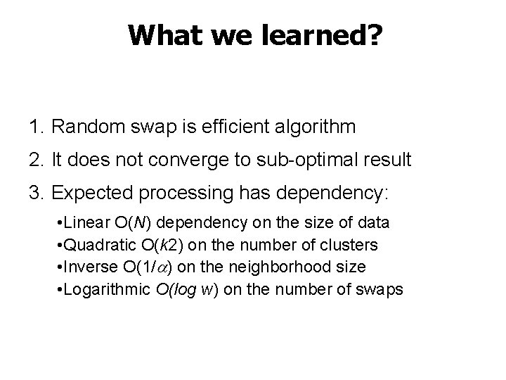
What we learned? 1. Random swap is efficient algorithm 2. It does not converge to sub-optimal result 3. Expected processing has dependency: • Linear O(N) dependency on the size of data • Quadratic O(k 2) on the number of clusters • Inverse O(1/ ) on the neighborhood size • Logarithmic O(log w) on the number of swaps

References • P. Fränti, "Efficiency of random swap clustering", Journal of Big Data, 5: 13, 1 -29, 2018. • P. Fränti and J. Kivijärvi, "Randomised local search algorithm for the clustering problem", Pattern Analysis and Applications, 3 (4), 358 -369, 2000. • P. Fränti, J. Kivijärvi and O. Nevalainen, "Tabu search algorithm for codebook generation in VQ", Pattern Recognition, 31 (8), 1139‑ 1148, August 1998. • P. Fränti, O. Virmajoki and V. Hautamäki, “Efficiency of random swap based clustering", IAPR Int. Conf. on Pattern Recognition (ICPR’ 08), Tampa, FL, Dec 2008. • Pseudo code: http: //cs. uef. fi/pages/franti/research/rs. txt

Supporting material Implementations available: (C, Matlab, Javascript, R and Python) http: //www. uef. fi/web/machine-learning/software Interactive animation: http: //cs. uef. fi/sipu/animator/ Clusterator: http: //cs. uef. fi/sipu/clusterator