Random Processes 1 Random variable A quantity X

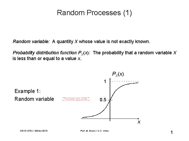
Random Processes (1) Random variable: A quantity X whose value is not exactly known. Probability distribution function PX(x): The probability that a random variable X is less than or equal to a value x. PX(x) 1 Example 1: Random variable 0. 5 x EECS 270 C / Winter 2013 Prof. M. Green / U. C. Irvine 1

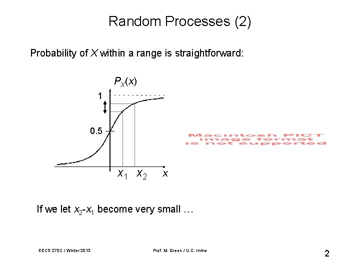
Random Processes (2) Probability of X within a range is straightforward: PX(x) 1 0. 5 x 1 x 2 x If we let x 2 -x 1 become very small … EECS 270 C / Winter 2013 Prof. M. Green / U. C. Irvine 2

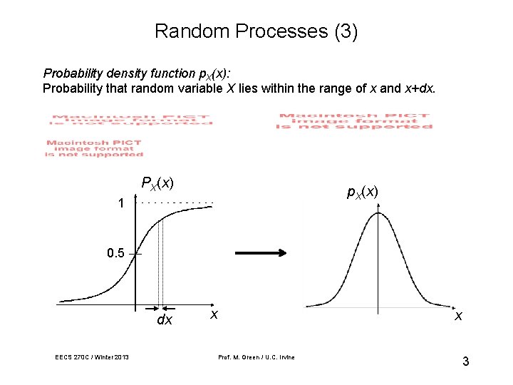
Random Processes (3) Probability density function p. X(x): Probability that random variable X lies within the range of x and x+dx. PX(x) p. X(x) 1 0. 5 dx EECS 270 C / Winter 2013 x x Prof. M. Green / U. C. Irvine 3

Random Processes (4) Expectation value E[X]: Expected (mean) value of random variable X over a large number of samples. Mean square value E[X 2]: Mean value of the square of a random variable X 2 over a large number of samples. Variance: Standard deviation: EECS 270 C / Winter 2013 Prof. M. Green / U. C. Irvine 4

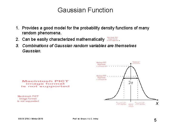
Gaussian Function 1. Provides a good model for the probability density functions of many random phenomena. 2. Can be easily characterized mathematically. 3. Combinations of Gaussian random variables are themselves Gaussian. 2 x EECS 270 C / Winter 2013 Prof. M. Green / U. C. Irvine 5

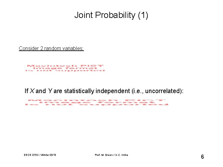
Joint Probability (1) Consider 2 random variables: If X and Y are statistically independent (i. e. , uncorrelated): EECS 270 C / Winter 2013 Prof. M. Green / U. C. Irvine 6

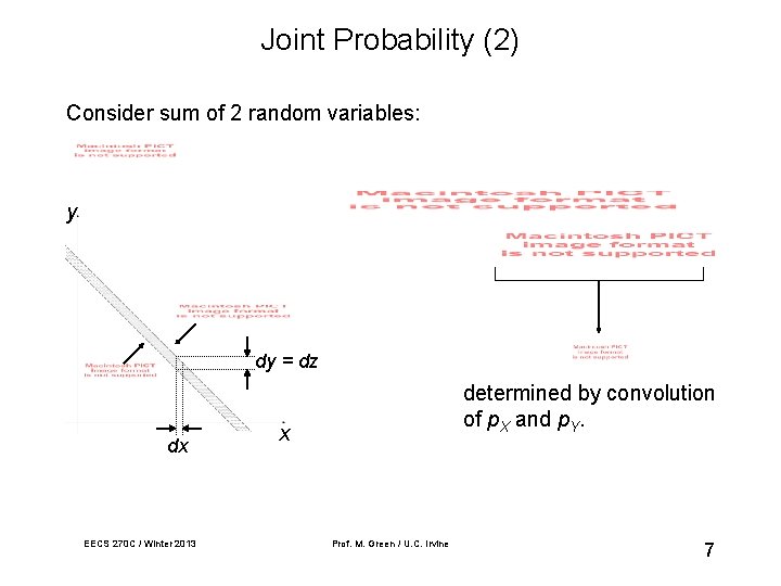
Joint Probability (2) Consider sum of 2 random variables: y dy = dz dx EECS 270 C / Winter 2013 determined by convolution of p. X and p. Y. x Prof. M. Green / U. C. Irvine 7

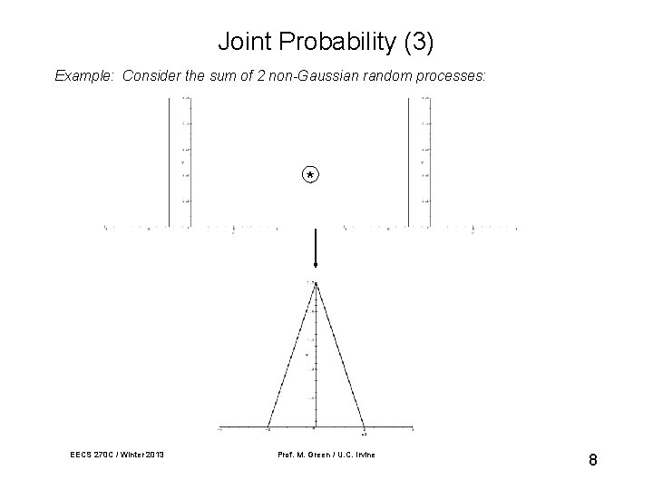
Joint Probability (3) Example: Consider the sum of 2 non-Gaussian random processes: * EECS 270 C / Winter 2013 Prof. M. Green / U. C. Irvine 8

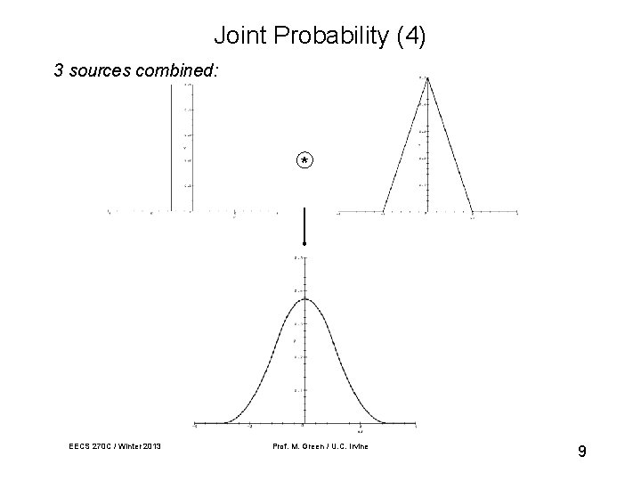
Joint Probability (4) 3 sources combined: * EECS 270 C / Winter 2013 Prof. M. Green / U. C. Irvine 9

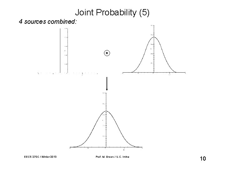
Joint Probability (5) 4 sources combined: * EECS 270 C / Winter 2013 Prof. M. Green / U. C. Irvine 10

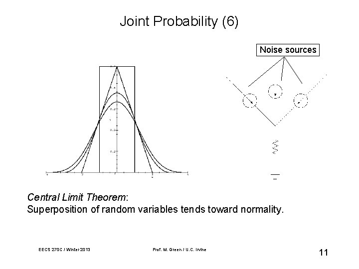
Joint Probability (6) Noise sources Central Limit Theorem: Superposition of random variables tends toward normality. EECS 270 C / Winter 2013 Prof. M. Green / U. C. Irvine 11

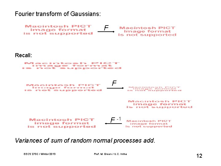
Fourier transform of Gaussians: F Recall: F F -1 Variances of sum of random normal processes add. EECS 270 C / Winter 2013 Prof. M. Green / U. C. Irvine 12

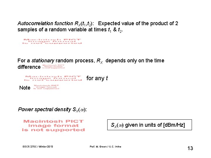
Autocorrelation function RX(t 1, t 2): Expected value of the product of 2 samples of a random variable at times t 1 & t 2. For a stationary random process, RX depends only on the time difference for any t Note Power spectral density SX( ): SX( ) given in units of [d. Bm/Hz] EECS 270 C / Winter 2013 Prof. M. Green / U. C. Irvine 13

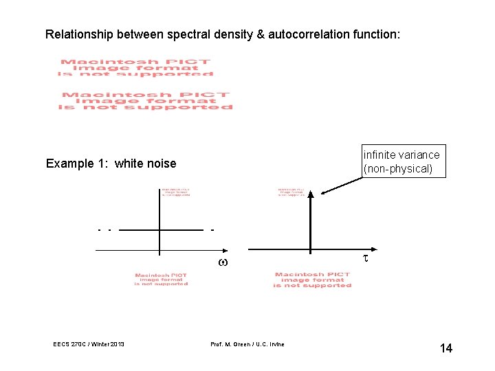
Relationship between spectral density & autocorrelation function: infinite variance (non-physical) Example 1: white noise EECS 270 C / Winter 2013 Prof. M. Green / U. C. Irvine 14

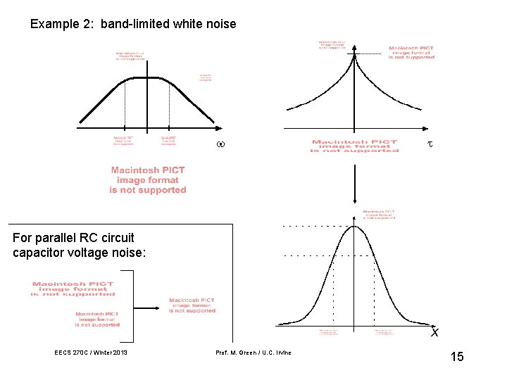
Example 2: band-limited white noise For parallel RC circuit capacitor voltage noise: x EECS 270 C / Winter 2013 Prof. M. Green / U. C. Irvine 15

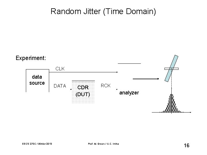
Random Jitter (Time Domain) Experiment: CLK data source EECS 270 C / Winter 2013 DATA CDR (DUT) RCK Prof. M. Green / U. C. Irvine analyzer 16

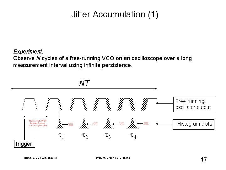
Jitter Accumulation (1) Experiment: Observe N cycles of a free-running VCO on an oscilloscope over a long measurement interval using infinite persistence. NT Free-running oscillator output Histogram plots 1 2 3 4 trigger EECS 270 C / Winter 2013 Prof. M. Green / U. C. Irvine 17

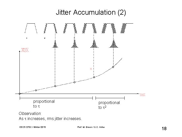
Jitter Accumulation (2) proportional to 2 Observation: As increases, rms jitter increases. EECS 270 C / Winter 2013 Prof. M. Green / U. C. Irvine 18

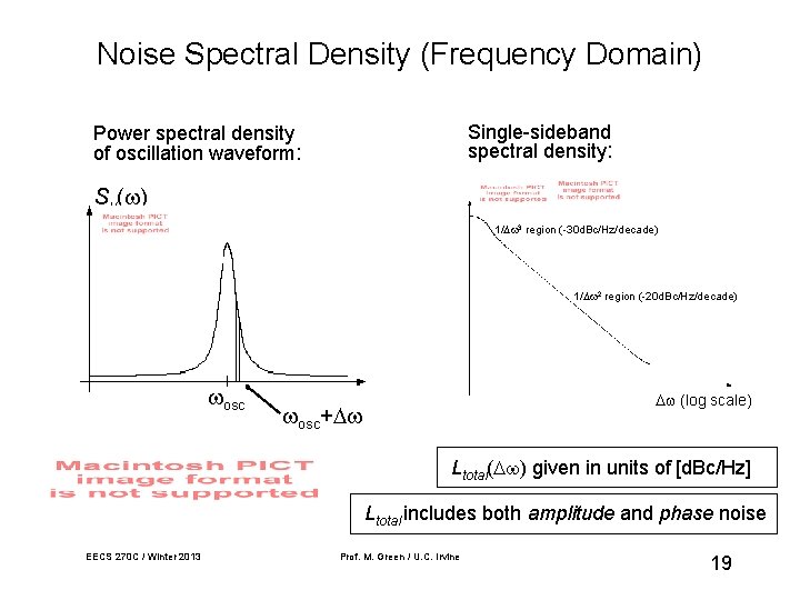
Noise Spectral Density (Frequency Domain) Single-sideband spectral density: Power spectral density of oscillation waveform: Sv( ) 1/ 3 region (-30 d. Bc/Hz/decade) 1/ 2 region (-20 d. Bc/Hz/decade) osc (log scale) osc+ Ltotal( ) given in units of [d. Bc/Hz] Ltotal includes both amplitude and phase noise EECS 270 C / Winter 2013 Prof. M. Green / U. C. Irvine 19

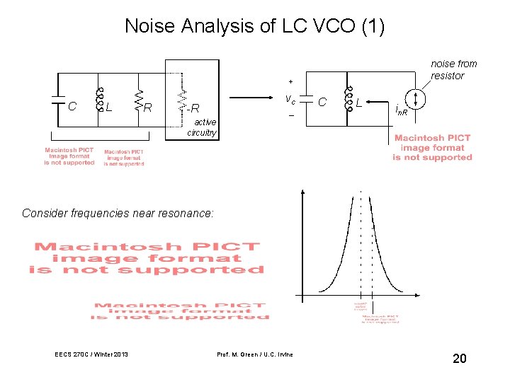
Noise Analysis of LC VCO (1) noise from resistor + C L R -R vc _ C L in. R active circuitry Consider frequencies near resonance: EECS 270 C / Winter 2013 Prof. M. Green / U. C. Irvine 20

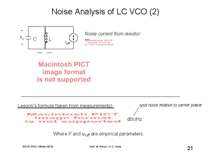
Noise Analysis of LC VCO (2) + vc _ Noise current from resistor: C L in. R Leeson’s formula (taken from measurements): spot noise relative to carrier power d. Bc/Hz Where F and 1/f 3 are empirical parameters. EECS 270 C / Winter 2013 Prof. M. Green / U. C. Irvine 21

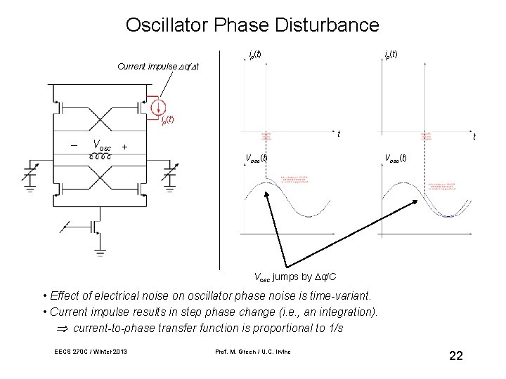
Oscillator Phase Disturbance ip(t) Current impulse q/ t ip(t) _ Vosc + t Vosc(t) Vosc jumps by q/C • Effect of electrical noise on oscillator phase noise is time-variant. • Current impulse results in step phase change (i. e. , an integration). current-to-phase transfer function is proportional to 1/s EECS 270 C / Winter 2013 Prof. M. Green / U. C. Irvine 22

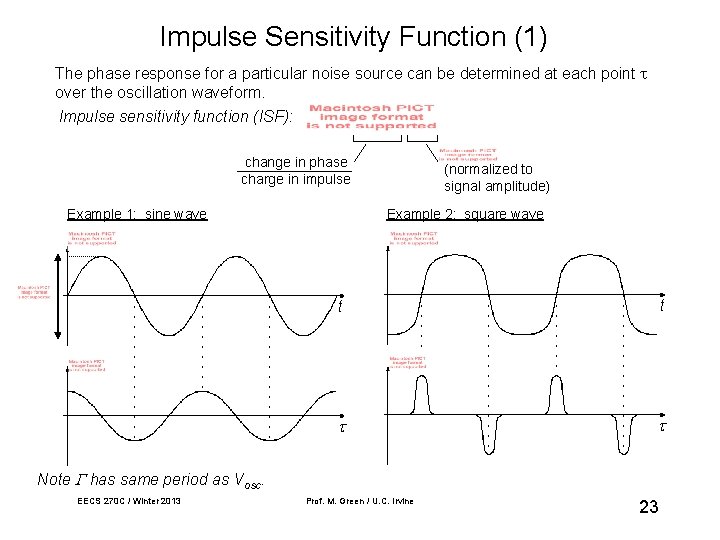
Impulse Sensitivity Function (1) The phase response for a particular noise source can be determined at each point over the oscillation waveform. Impulse sensitivity function (ISF): change in phase charge in impulse Example 1: sine wave (normalized to signal amplitude) Example 2: square wave t t Note has same period as Vosc. EECS 270 C / Winter 2013 Prof. M. Green / U. C. Irvine 23

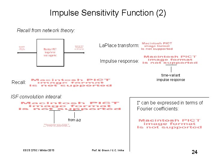
Impulse Sensitivity Function (2) Recall from network theory: La. Place transform: Impulse response: time-variant impulse response Recall: ISF convolution integral: can be expressed in terms of Fourier coefficients: from q EECS 270 C / Winter 2013 Prof. M. Green / U. C. Irvine 24

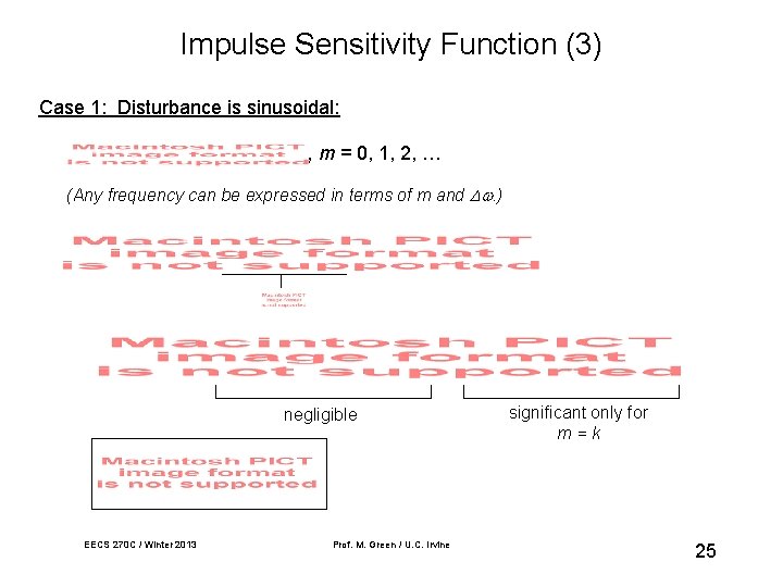
Impulse Sensitivity Function (3) Case 1: Disturbance is sinusoidal: , m = 0, 1, 2, … (Any frequency can be expressed in terms of m and . ) negligible EECS 270 C / Winter 2013 Prof. M. Green / U. C. Irvine significant only for m=k 25

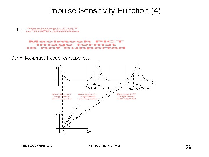
Impulse Sensitivity Function (4) For Current-to-phase frequency response: I osc osc 2 osc EECS 270 C / Winter 2013 Prof. M. Green / U. C. Irvine 26

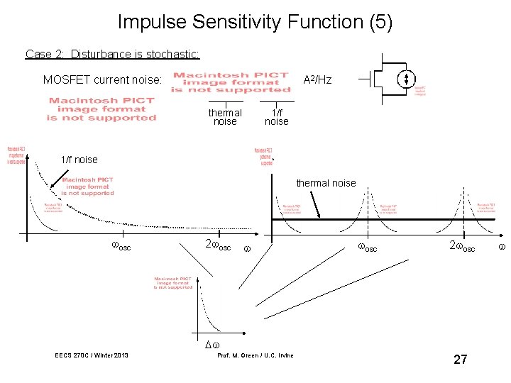
Impulse Sensitivity Function (5) Case 2: Disturbance is stochastic: MOSFET current noise: A 2/Hz thermal noise 1/f noise thermal noise osc 2 osc EECS 270 C / Winter 2013 Prof. M. Green / U. C. Irvine 27

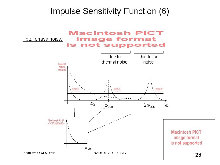
Impulse Sensitivity Function (6) Total phase noise: due to thermal noise n osc due to 1/f noise 2 osc EECS 270 C / Winter 2013 Prof. M. Green / U. C. Irvine 28

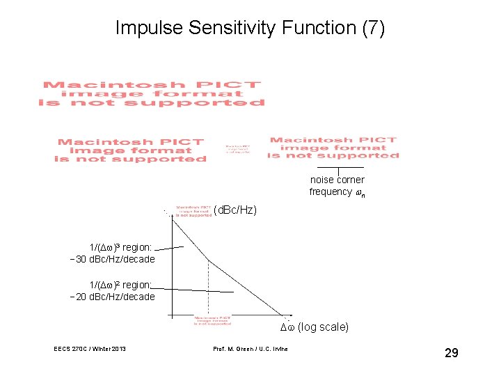
Impulse Sensitivity Function (7) noise corner frequency n (d. Bc/Hz) 1/( 3 region: − 30 d. Bc/Hz/decade 1/( 2 region: − 20 d. Bc/Hz/decade (log scale) EECS 270 C / Winter 2013 Prof. M. Green / U. C. Irvine 29

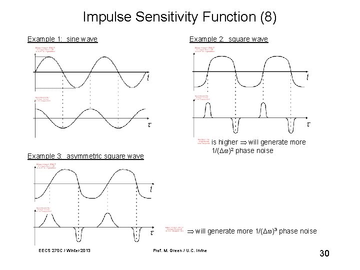
Impulse Sensitivity Function (8) Example 1: sine wave Example 2: square wave t t is higher will generate more 1/( 2 phase noise Example 3: asymmetric square wave t EECS 270 C / Winter 2013 will generate more 1/( 3 phase noise Prof. M. Green / U. C. Irvine 30

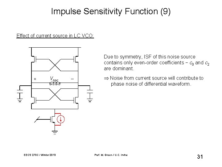
Impulse Sensitivity Function (9) Effect of current source in LC VCO: Due to symmetry, ISF of this noise source contains only even-order coefficients − c 0 and c 2 are dominant. + Vosc EECS 270 C / Winter 2013 _ Noise from current source will contribute to phase noise of differential waveform. Prof. M. Green / U. C. Irvine 31

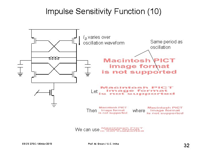
Impulse Sensitivity Function (10) ID varies over oscillation waveform Same period as oscillation Let Then where We can use EECS 270 C / Winter 2013 Prof. M. Green / U. C. Irvine 32

ISF Example: 3 -Stage Ring Oscillator R 1 A R 1 B M 1 A M 1 B MS 1 R 2 A R 2 B M 2 A M 2 B MS 2 R 3 A R 3 B M 3 A + Vout − M 3 B MS 3 Red curve: Unperturbed oscillation waveform Blue curve: Oscillation waveform perturbed by impulse fosc = 1. 08 GHz PD = 11 m. W EECS 270 C / Winter 2013 Prof. M. Green / U. C. Irvine 33

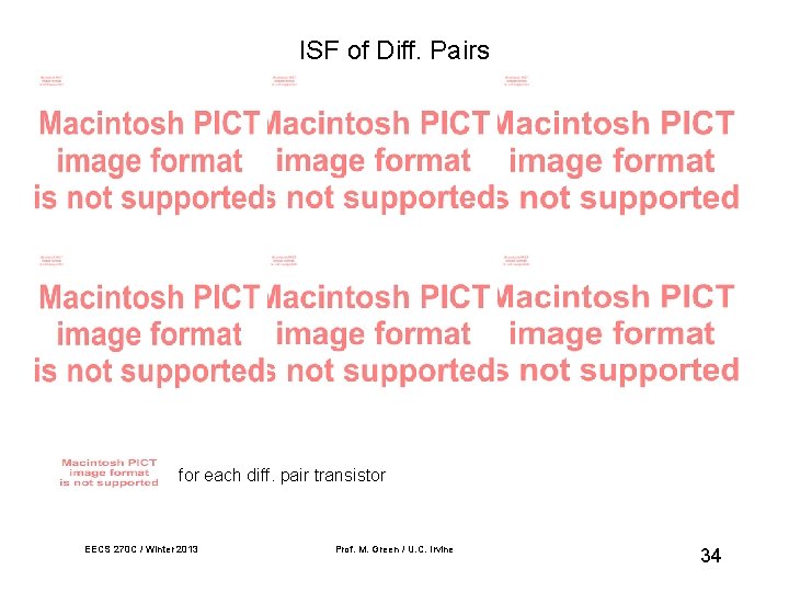
ISF of Diff. Pairs for each diff. pair transistor EECS 270 C / Winter 2013 Prof. M. Green / U. C. Irvine 34

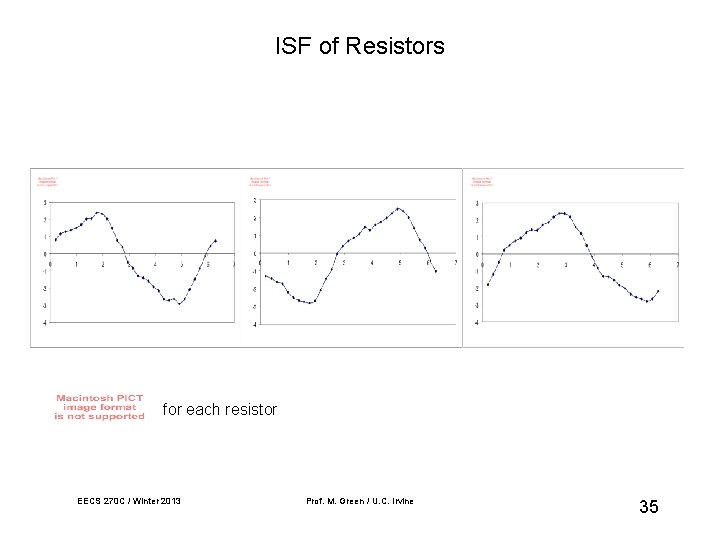
ISF of Resistors for each resistor EECS 270 C / Winter 2013 Prof. M. Green / U. C. Irvine 35

ISF of Current Sources for each current source transistor ISF shows double frequency due to source-coupled node connection. EECS 270 C / Winter 2013 Prof. M. Green / U. C. Irvine 36

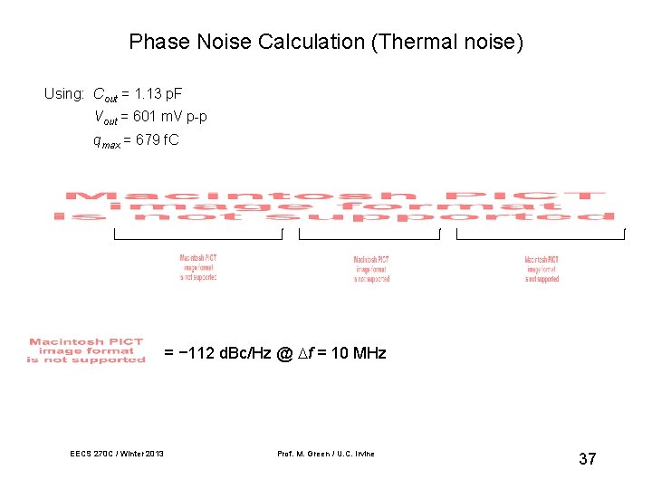
Phase Noise Calculation (Thermal noise) Using: Cout = 1. 13 p. F Vout = 601 m. V p-p qmax = 679 f. C = − 112 d. Bc/Hz @ f = 10 MHz EECS 270 C / Winter 2013 Prof. M. Green / U. C. Irvine 37

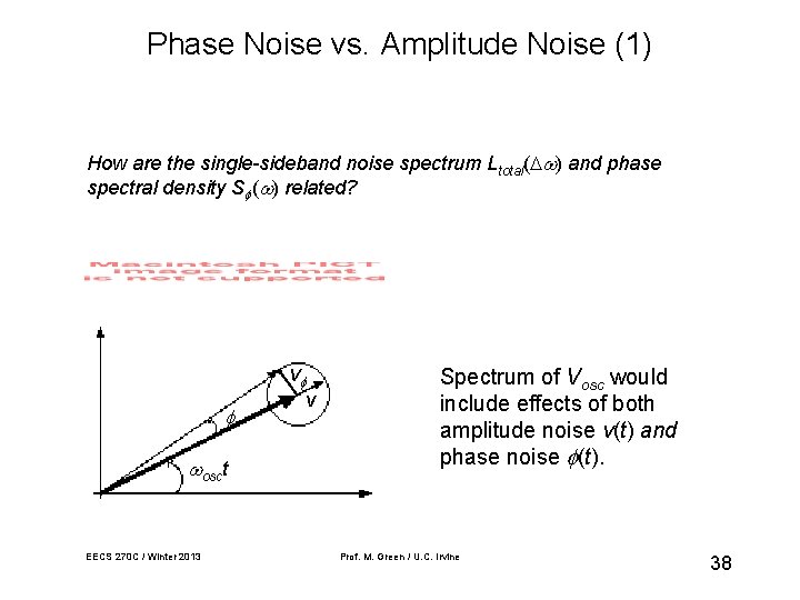
Phase Noise vs. Amplitude Noise (1) How are the single-sideband noise spectrum Ltotal( ) and phase spectral density S ( ) related? v osct EECS 270 C / Winter 2013 v Spectrum of Vosc would include effects of both amplitude noise v(t) and phase noise (t). Prof. M. Green / U. C. Irvine 38

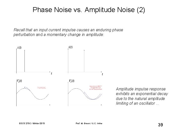
Phase Noise vs. Amplitude Noise (2) Recall that an input current impulse causes an enduring phase perturbation and a momentary change in amplitude: i(t) t Vc(t) Amplitude impulse response exhibits an exponential decay due to the natural amplitude limiting of an oscillator. . . EECS 270 C / Winter 2013 Prof. M. Green / U. C. Irvine 39

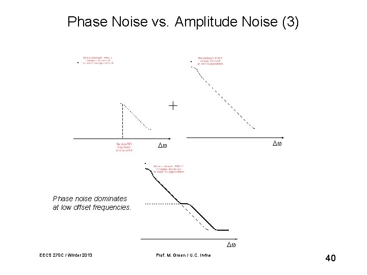
Phase Noise vs. Amplitude Noise (3) + Phase noise dominates at low offset frequencies. EECS 270 C / Winter 2013 Prof. M. Green / U. C. Irvine 40

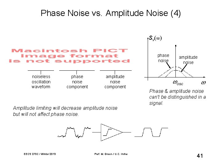
Phase Noise vs. Amplitude Noise (4) Sv( ) phase noiseless oscillation waveform phase noise component amplitude noise component Amplitude limiting will decrease amplitude noise but will not affect phase noise. EECS 270 C / Winter 2013 Prof. M. Green / U. C. Irvine amplitude noise osc Phase & amplitude noise can’t be distinguished in a signal. 41

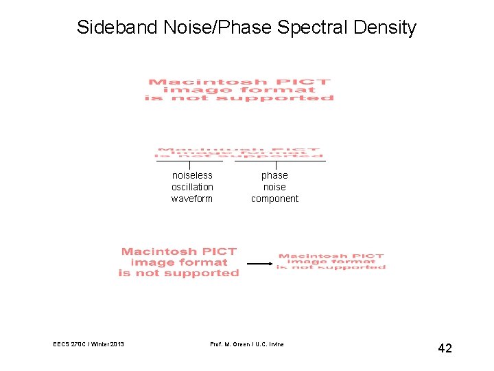
Sideband Noise/Phase Spectral Density noiseless oscillation waveform EECS 270 C / Winter 2013 phase noise component Prof. M. Green / U. C. Irvine 42

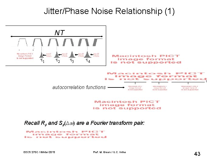
Jitter/Phase Noise Relationship (1) NT 1 2 3 4 autocorrelation functions Recall R and S ( ) are a Fourier transform pair: EECS 270 C / Winter 2013 Prof. M. Green / U. C. Irvine 43

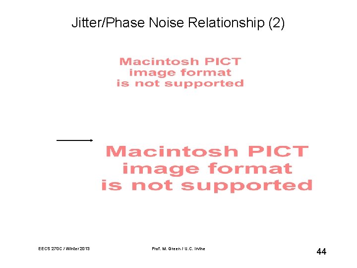
Jitter/Phase Noise Relationship (2) EECS 270 C / Winter 2013 Prof. M. Green / U. C. Irvine 44

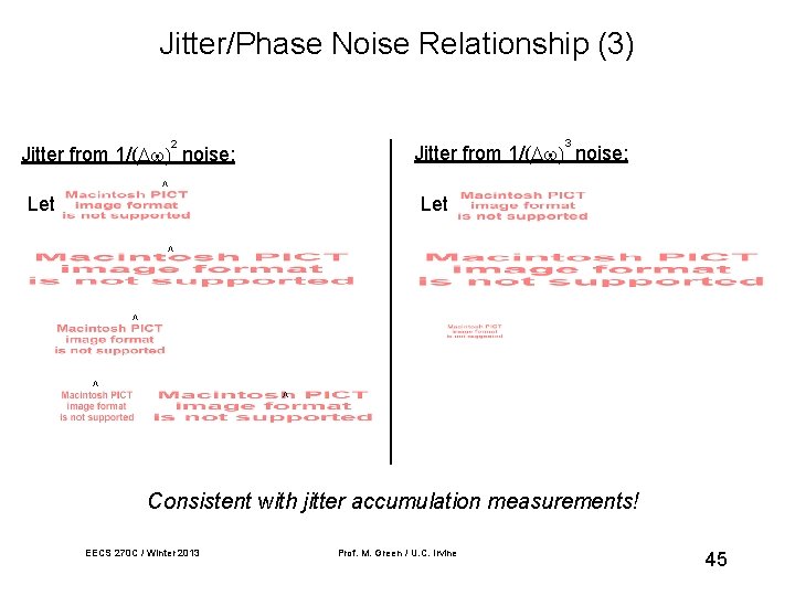
Jitter/Phase Noise Relationship (3) 3 2 Jitter from 1/( noise: ^ Let ^ ^ Consistent with jitter accumulation measurements! EECS 270 C / Winter 2013 Prof. M. Green / U. C. Irvine 45

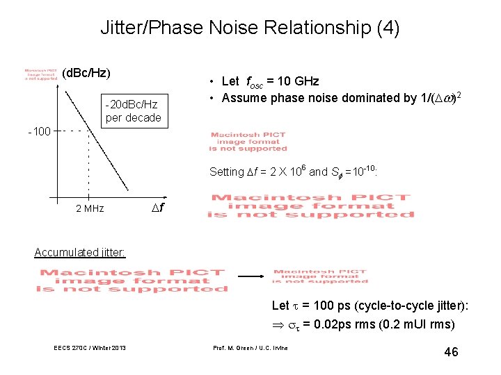
Jitter/Phase Noise Relationship (4) (d. Bc/Hz) -20 d. Bc/Hz per decade • Let fosc = 10 GHz • Assume phase noise dominated by 1/( )2 -100 Setting f = 2 X 106 and S =10 -10: 2 MHz f Accumulated jitter: Let = 100 ps (cycle-to-cycle jitter): = 0. 02 ps rms (0. 2 m. UI rms) EECS 270 C / Winter 2013 Prof. M. Green / U. C. Irvine 46

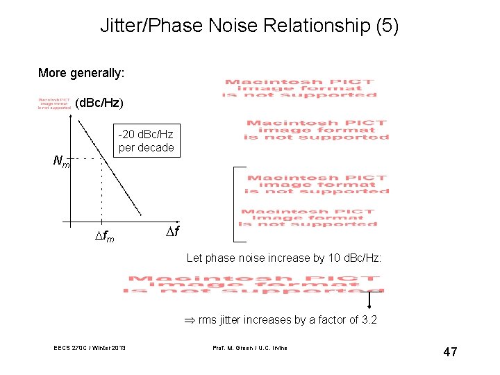
Jitter/Phase Noise Relationship (5) More generally: (d. Bc/Hz) -20 d. Bc/Hz per decade Nm f Let phase noise increase by 10 d. Bc/Hz: rms jitter increases by a factor of 3. 2 EECS 270 C / Winter 2013 Prof. M. Green / U. C. Irvine 47

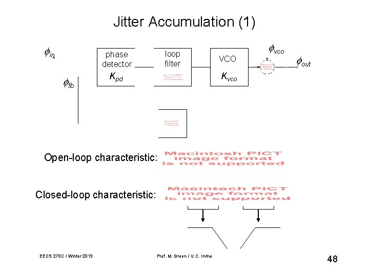
Jitter Accumulation (1) in loop filter phase detector fb Kpd VCO vco out Kvco Open-loop characteristic: Closed-loop characteristic: EECS 270 C / Winter 2013 Prof. M. Green / U. C. Irvine 48

Jitter Accumulation (2) Recall from Type-2 PLL: -40 d. B/decade (d. Bc/Hz) |1 + G| 1/( 3 region: − 30 d. Bc/Hz/decade |G| z p 1/( 2 region: − 20 d. Bc/Hz/decade 1 As a result, the phase noise at low offset frequencies is determined by input noise. . . 80 d. B/decade EECS 270 C / Winter 2013 Prof. M. Green / U. C. Irvine 49

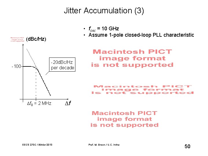
Jitter Accumulation (3) • fosc = 10 GHz • Assume 1 -pole closed-loop PLL characteristic (d. Bc/Hz) -100 -20 d. Bc/Hz per decade f 0 = 2 MHz EECS 270 C / Winter 2013 f Prof. M. Green / U. C. Irvine 50

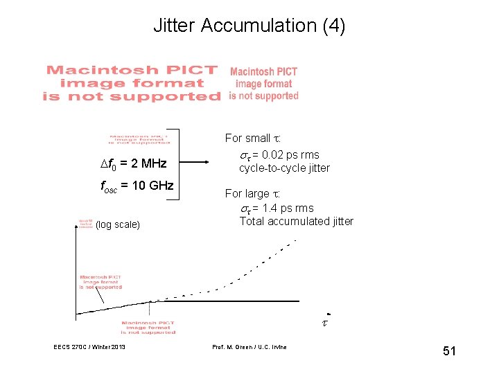
Jitter Accumulation (4) f 0 = 2 MHz fosc = 10 GHz (log scale) For small : = 0. 02 ps rms cycle-to-cycle jitter For large : = 1. 4 ps rms Total accumulated jitter EECS 270 C / Winter 2013 Prof. M. Green / U. C. Irvine 51

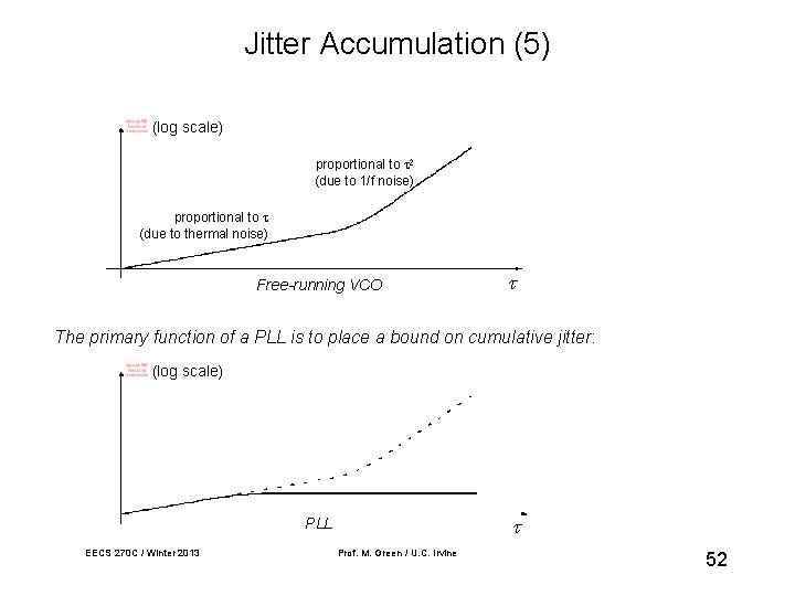
Jitter Accumulation (5) (log scale) proportional to (due to 1/f noise) proportional to (due to thermal noise) Free-running VCO The primary function of a PLL is to place a bound on cumulative jitter: (log scale) PLL EECS 270 C / Winter 2013 Prof. M. Green / U. C. Irvine 52

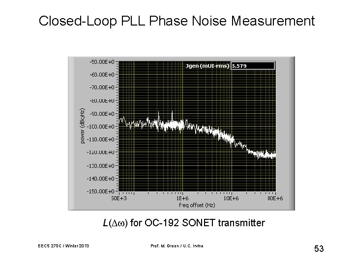
Closed-Loop PLL Phase Noise Measurement L( ) for OC-192 SONET transmitter EECS 270 C / Winter 2013 Prof. M. Green / U. C. Irvine 53

Other Sources of Jitter in PLL • Clock divider • Phase detector Ripple on phase detector output can cause high-frequency jitter. This affects primarily the jitter tolerance of CDR. EECS 270 C / Winter 2013 Prof. M. Green / U. C. Irvine 54

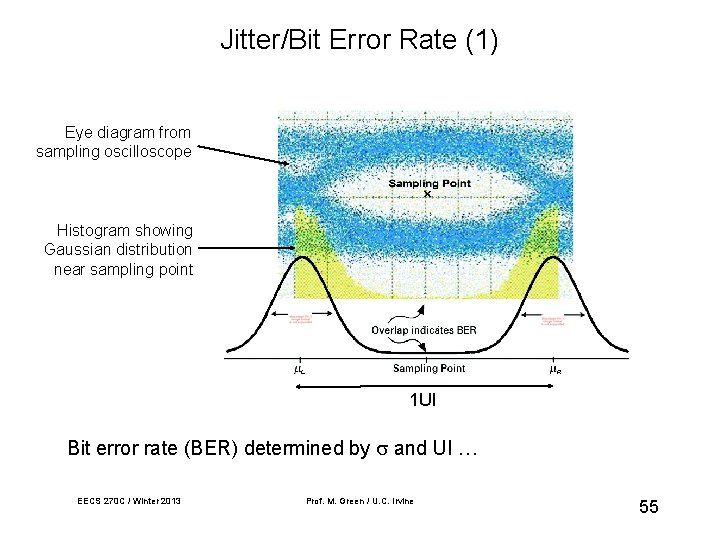
Jitter/Bit Error Rate (1) Eye diagram from sampling oscilloscope Histogram showing Gaussian distribution near sampling point L R 1 UI Bit error rate (BER) determined by and UI … EECS 270 C / Winter 2013 Prof. M. Green / U. C. Irvine 55

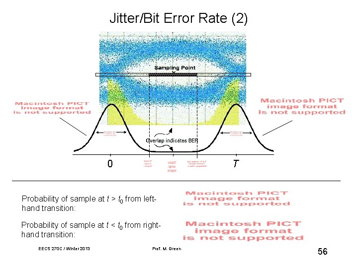
Jitter/Bit Error Rate (2) 0 T R Probability of sample at t > t 0 from lefthand transition: Probability of sample at t < t 0 from righthand transition: EECS 270 C / Winter 2013 Prof. M. Green / U. C. Irvine 56

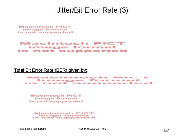
Jitter/Bit Error Rate (3) Total Bit Error Rate (BER) given by: EECS 270 C / Winter 2013 Prof. M. Green / U. C. Irvine 57

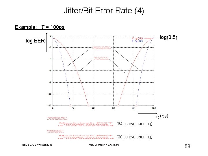
Jitter/Bit Error Rate (4) Example: T = 100 ps log(0. 5) log BER t 0 (ps) (64 ps eye opening) (38 ps eye opening) EECS 270 C / Winter 2013 Prof. M. Green / U. C. Irvine 58

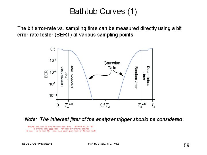
Bathtub Curves (1) The bit error-rate vs. sampling time can be measured directly using a bit error-rate tester (BERT) at various sampling points. Note: The inherent jitter of the analyzer trigger should be considered. EECS 270 C / Winter 2013 Prof. M. Green / U. C. Irvine 59

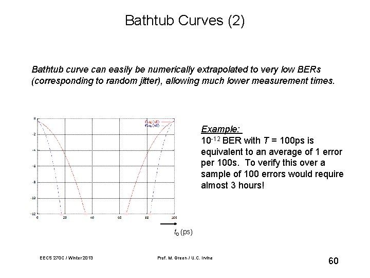
Bathtub Curves (2) Bathtub curve can easily be numerically extrapolated to very low BERs (corresponding to random jitter), allowing much lower measurement times. Example: 10 -12 BER with T = 100 ps is equivalent to an average of 1 error per 100 s. To verify this over a sample of 100 errors would require almost 3 hours! t 0 (ps) EECS 270 C / Winter 2013 Prof. M. Green / U. C. Irvine 60

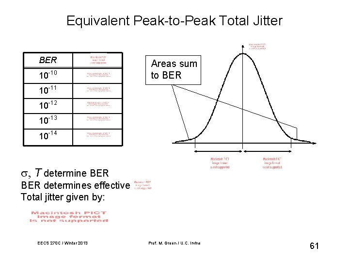
Equivalent Peak-to-Peak Total Jitter BER 10 -10 Areas sum to BER 10 -11 10 -12 10 -13 10 -14 , T determine BER determines effective Total jitter given by: EECS 270 C / Winter 2013 Prof. M. Green / U. C. Irvine 61