Random Field Theory Mkael Symmonds Bahador Bahrami Random

Random Field Theory Mkael Symmonds, Bahador Bahrami

Random Field Theory Mkael Symmonds, Bahador Bahrami

Overview n Spatial smoothing n Statistical inference n The multiple comparison problem n …and what to do about it

Overview n Spatial smoothing n Statistical inference n The multiple comparison problem n …and what to do about it

Statistical inference n Aim – to decide if the data represents convincing evidence of the effect we are interested in. n How – perform a statistical test across the whole brain volume to tell us how likely our data are to have come about by chance (the null distribution).

Inference at a single voxel NULL hypothesis, H 0: activation is zero t-distribution t-value = 2. 42 p-value: probability of getting a value of t at least as extreme as 2. 42 from the t distribution (= 0. 01). a = p(t>t-value|H 0) t-value = 2. 02 t-value = 2. 42 alpha = 0. 025 As p < α , we reject the null hypothesis

Sensitivity and Specificity ACTION Don’t Reject Chance H 0 True TN FP – type I error Not by chance H 0 False FN TP Specificity = TN/(# H True) = TN/(TN+FP) = 1 - a Sensitivity = TP/(# H False) = TP/(TP+FN) = b = power

Many statistical tests n In functional imaging, there are many voxels, therefore many statistical tests n If we do not know where in the brain our effect will occur, the hypothesis relates to the whole volume of statistics in the brain n n We would reject H 0 if the entire family of statistical values is unlikely to have arisen from a null distribution – a familywise hypothesis The risk of error we are prepared to accept is called the Family-Wise Error (FWE) rate – what is the likelihood that the family of voxel values could have arisen by chance

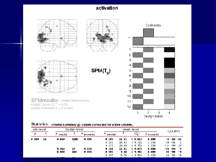
How to test a family-wise hypothesis? Height thresholding This can localise significant test results

How to set the threshold? n Should we use the same alpha as when we perform inference at a single voxel?

Overview n Spatial smoothing n Statistical inference n The multiple comparison problem n …and what to do about it

How to set the threshold? Signal + Noise Use of ‘uncorrected’ alpha, a=0. 1 11. 3% 12. 5% 10. 8% 11. 5% 10. 0% 10. 7% 11. 2% Percentage of Null Pixels that are False Positives 10. 2% LOTS OF SIGNIFICANT ACTIVATIONS OUTSIDE OF OUR SIGNAL BLOB! 9. 5%

How to set the threshold? n So, if we see 1 t-value above our uncorrected threshold in the family of tests, this is not good evidence against the family- wise null hypothesis n If we are prepared to accept a false positive rate of 5%, we need a threshold such that, for the entire family of statistical tests, there is a 5% chance of there being one or more t values above that threshold.
 – Probability")
Bonferroni Correction n For one voxel (all values from a null distribution) – Probability of a result greater than the threshold = α – Probability of a result less than the threshold = 1 -α 1 n For n voxels (all values from a null distribution) – Probability of all n results being less than the threshold = (1 -α) (1 - n – Probability of one (or more) tests being greater than the threshold: = 1 -(1 -α) (1 - n ~= n. α (as alpha is small) FAMILY WISE ERROR RATE

Bonferroni Correction n So, n Set the PFWE < n. α n. Gives a threshold α = PFWE / n n n Should we use the Bonferroni correction for imaging data?

100 x 100 voxels – normally distributed independent random numbers 10, 000 tests 5% FWE rate Apply Bonferroni correction to give threshold of 0. 05/10000 = 0. 000005 This corresponds to a z-score of 4. 42 We expect only 5 out of 100 such images to have one or more z-scores > 4. 42 NULL HYPOTHESIS TRUE 100 x 100 voxels averaged Now only 10 x 10 independent numbers in our image The appropriate Bonferroni correction is 0. 05/100= 0. 0005 This corresponds to z-score = 3. 29 Only 5/100 such images will have one or more z-scores > 3. 29 by chance

Spatial correlation Physiological Correlation Spatial pre-processing Smoothing Assumes Independent Voxels Spatially Correlated Voxels Bonferroni is too conservative for brain images, but how to tell how many independent observations there are?

Overview n Spatial smoothing n Statistical inference n The multiple comparison problem n …and what to do about it

Spatial smoothing Why do you want to do it? n Increases signal-to-noise ratio n Enables averaging across subjects n Allows use of Gaussian Random Field Theory for thresholding

Spatial Smoothing What does it do? n Reduces effect of high frequency variation in functional imaging data, “blurring sharp edges”

Spatial Smoothing How is it done? n Typically in functional imaging, a Gaussian smoothing kernel is used – Shape similar to normal distribution bell curve – Width usually described using “full width at half maximum” (FWHM) measure e. g. , for kernel at 10 mm FWHM: -5 0 5

Spatial Smoothing How is it done? n Gaussian kernel defines shape of function used successively to calculate weighted average of each data point with respect to its neighbouring data points Raw data x Gaussian function = Smoothed data

Spatial Smoothing How is it done? n Gaussian kernel defines shape of function used successively to calculate weighted average of each data point with respect to its neighbouring data points Raw data x Gaussian function = Smoothed data

Spatial correlation Physiological Correlation Spatial pre-processing Smoothing Assumes Independent Voxels Spatially Correlated Voxels Bonferroni is too conservative for brain images, but how to tell how many independent observations there are?

Overview n Spatial smoothing n Statistical inference n The multiple comparison problem n …and what to do about it
 Methods for Dummies 2008 Mkael Symmonds Bahador Bahrami")
Random Field Theory (ii) Methods for Dummies 2008 Mkael Symmonds Bahador Bahrami

What is a random field? n A random field is a list of random numbers whose values are mapped onto a space (of n dimensions). Values in a random field are usually spatially correlated in one way or another, in its most basic form this might mean that adjacent values do not differ as much as values that are further apart.

Why random field? n To characterise the properties our study’s statistical parametric map under the NULL hypothesis – NULL hypothesis = n if all predictions were wrong n all activations were merely driven by chance n each voxel value was a random number – What would the probability of getting a certain z-score for a voxel in this situation be?

Random Field

Thresholded @ one Thresholded @ Zero

Measurement 1 Thresholded @ three Number of blobs = 4 Measurement 2 Number of blobs = 0 Measurement 3 Number of blobs = 1 Number of blobs = 2 Measurement 100000 Average number of blobs = (4 + 0 + 1 + … + 2)/100000 The probability of getting a z-score>3 by chance

Therefore, for every z-score, the expected value of number of blobs = probability of rejecting the null hypothesis erroneously (α)

The million-dollar question is: thresholding the random field at which Zscore produces average number of blobs < 0. 05? n Or, Which Z-score has a probability = 0. 05 of rejecting the null hypothesis erroneously? n – Any z-scores above that will be significant!

So, it all comes down to estimating the average number of blobs (that you expect by chance) in your SPM Random field theory does that for you!

Expected number of blobs in a random field depends on … n Chosen threshold z-score n Volume of search region Roughness (i. e. , 1/smoothness) of the search region: Spatial extent of correlation among values in the field; it is described by FWHM n – Volume and Roughness are combined into RESELs – Where does SPM get R from: it is calculated from the residuals (RPV. img) – Given the R and Z, RFT calculates the expected number of blobs for you: E(EC) = R (4 ln 2) (2π) -3/2 z exp(-z 2/2)

Probability of Family Wise Error PFWE = average number of blobs under null hypothesis α = PFWE = R (4 ln 2) (2π) -3/2 z exp(-z 2/2)

Thank you n References: – Brett, Penny & Keibel. An introduction to Random Field Theory. Chapter from Human Brain Mapping – Will Penny’s slides (http: //www. fil. ion. ucl. ac. uk/spm/course/slides 0 5/ppt/infer. ppt#324, 1, Random Field Theory) – Jean-Etienne Poirrier’s slides (http: //www. poirrier. be/~jeanetienne/presentations/rft/spm-rft-slidespoirrier 06. pdf) – Tom Nichol’s lecture in SPM Short Course (2006)
")
False Discovery Rate ACTION Don’t Reject TRUTH At u 1 Reject H True (o) TN=7 FP=3 H False (x) FN=0 TP=10 Eg. t-scores from regions that truly do and do not activate FDR = FP/(# Reject) a = FP/(# H True) FDR=3/13=23% a=3/10=30% oooooooxxxoxxxx u 1

False Discovery Rate ACTION Don’t Reject TRUTH At u 2 Reject FDR=1/8=13% a=1/10=10% H True (o) TN=9 FP=1 H False (x) FN=3 TP=7 Eg. t-scores from regions that truly do and do not activate FDR = FP/(# Reject) a = FP/(# H True) oooooooxxxoxxxx u 2

False Discovery Rate Noise Signal+Noise

Control of Familywise Error Rate at 10% Occurrence of Familywise Error FWE Control of False Discovery Rate at 10% 6. 7% 10. 4% 14. 9% 9. 3% 16. 2% 13. 8% 14. 0% 10. 5% 12. 2% Percentage of Activated Pixels that are False Positives 8. 7%

Cluster Level Inference n We can increase sensitivity by trading off anatomical specificity n Given a voxel level threshold u, we can compute the likelihood (under the null hypothesis) of getting a cluster containing at least n voxels CLUSTER-LEVEL INFERENCE n Similarly, we can compute the likelihood of getting c clusters each having at least n voxels
 =")
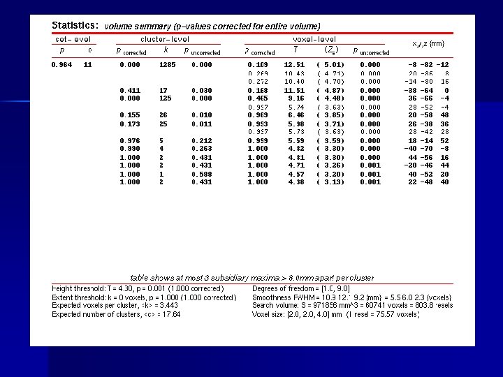
Levels of inference voxel-level P(c 1 | n > 0, t 4. 37) = 0. 048 (corrected) At least one cluster with unspecified number of voxels above threshold n=1 2 n=82 set-level P(c 3 | n 12, u 3. 09) = At least 3 0. 019 clusters above threshold n=32 cluster-level P(c 1 | n 82, t 3. 09) = 0. 029 (corrected) At least one cluster with at least 82 voxels above threshold
- Slides: 45