Random Effects Repeated Measures Alternatives to Fixed Effects

Random Effects & Repeated Measures Alternatives to Fixed Effects Analyses

Questions q What is the difference between fixed- and random-effects in terms of treatments? q How are F tests with random effects different than with fixed effects? q Describe a concrete example of a randomized block design. You should have 1 factor as the blocking factor and one other factor as the factor of main interest.

Questions (2) q q q How is a repeated measures design different from a totally between subjects design in the collection of the data? How does the significance testing change from the totally between to a design to one in which one or more factors are repeated measures (just the general idea, you don’t need to show actual F ratios or computations)? Describe one argument for using repeated measures designs and one argument against using such designs (or describe when you would and would not want to use repeated measures).

Fixed Effects Designs • All treatment conditions of interest are included in the study • All in cell get identical stimulus (treatment, IV combination) • Interest is in specific means • Expected mean squares are (relatively) simple; F tests are all based on common error term.

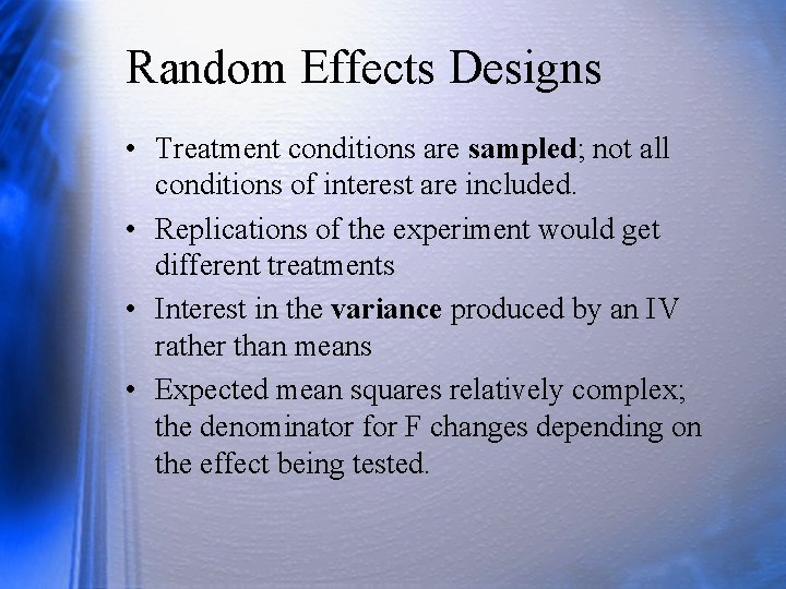
Random Effects Designs • Treatment conditions are sampled; not all conditions of interest are included. • Replications of the experiment would get different treatments • Interest in the variance produced by an IV rather than means • Expected mean squares relatively complex; the denominator for F changes depending on the effect being tested.

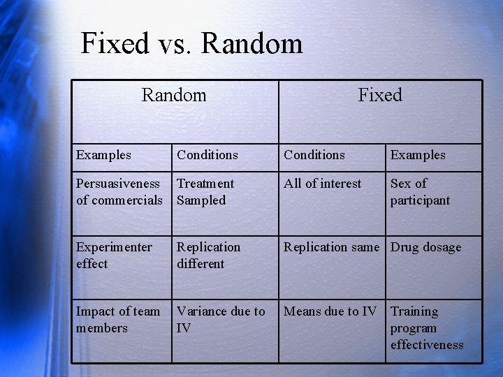
Fixed vs. Random Fixed Examples Conditions Examples Persuasiveness of commercials Treatment Sampled All of interest Sex of participant Experimenter effect Replication different Replication same Drug dosage Impact of team members Variance due to IV Means due to IV Training program effectiveness

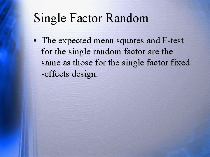
Single Factor Random • The expected mean squares and F-test for the single random factor are the same as those for the single factor fixed -effects design.

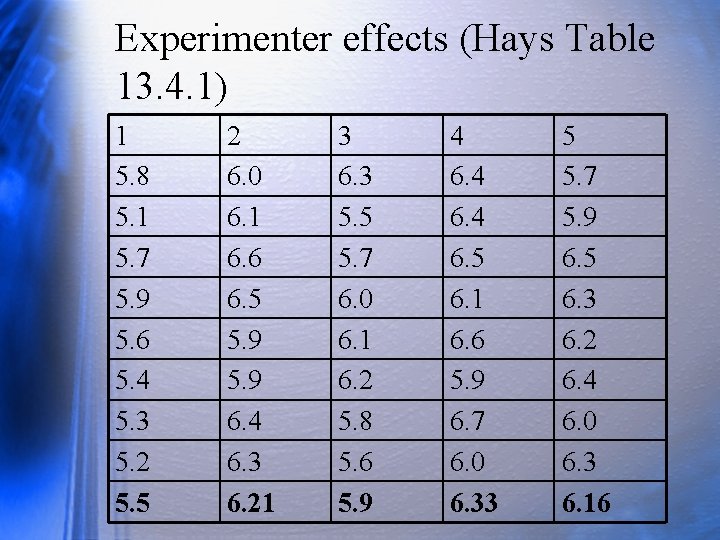
Experimenter effects (Hays Table 13. 4. 1) 1 5. 8 5. 1 5. 7 5. 9 5. 6 5. 4 5. 3 5. 2 5. 5 2 6. 0 6. 1 6. 6 6. 5 5. 9 6. 4 6. 3 6. 21 3 6. 3 5. 5 5. 7 6. 0 6. 1 6. 2 5. 8 5. 6 5. 9 4 6. 5 6. 1 6. 6 5. 9 6. 7 6. 0 6. 33 5 5. 7 5. 9 6. 5 6. 3 6. 2 6. 4 6. 0 6. 3 6. 16

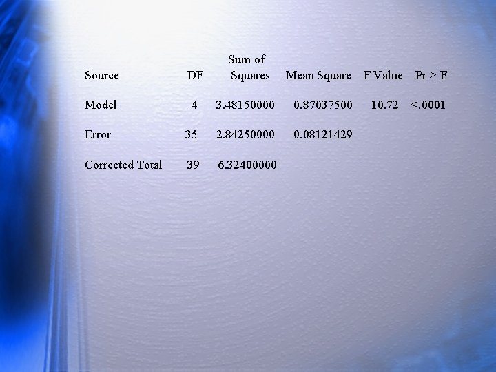
Source DF Sum of Squares Model 4 3. 48150000 0. 87037500 Error 35 2. 84250000 0. 08121429 Corrected Total 39 6. 32400000 Mean Square F Value Pr > F 10. 72 <. 0001

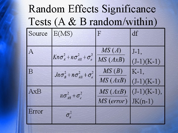
Random Effects Significance Tests (A & B random/within) Source E(MS) A B Ax. B Error F df J-1, (J-1)(K-1) K-1, (J-1)(K-1), JK(n-1)

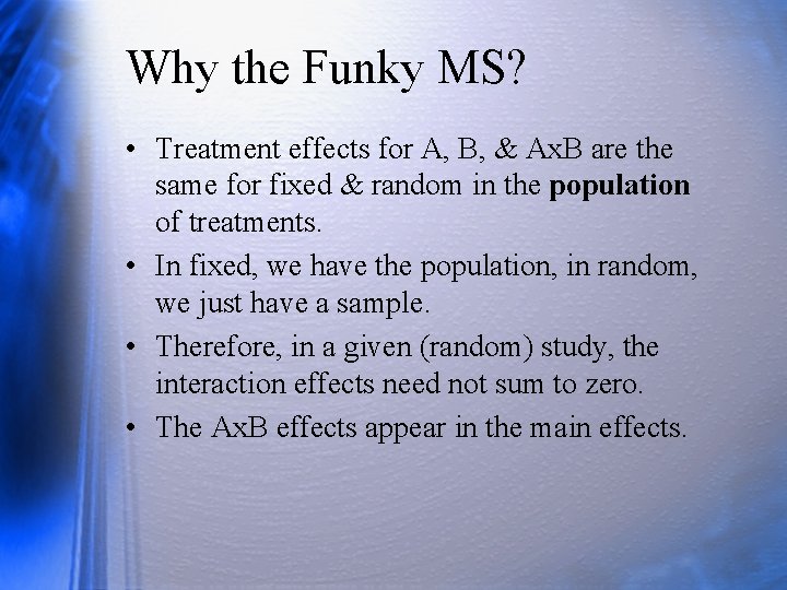
Why the Funky MS? • Treatment effects for A, B, & Ax. B are the same for fixed & random in the population of treatments. • In fixed, we have the population, in random, we just have a sample. • Therefore, in a given (random) study, the interaction effects need not sum to zero. • The Ax. B effects appear in the main effects.

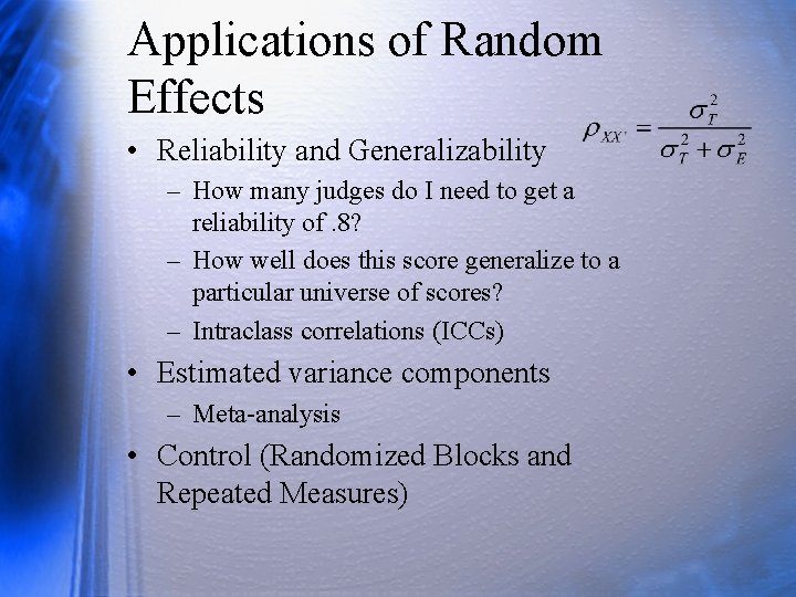
Applications of Random Effects • Reliability and Generalizability – How many judges do I need to get a reliability of. 8? – How well does this score generalize to a particular universe of scores? – Intraclass correlations (ICCs) • Estimated variance components – Meta-analysis • Control (Randomized Blocks and Repeated Measures)

Review q. What is the difference between fixedand random-effects in terms of treatments? q. How are F tests with random effects different than with fixed effects?

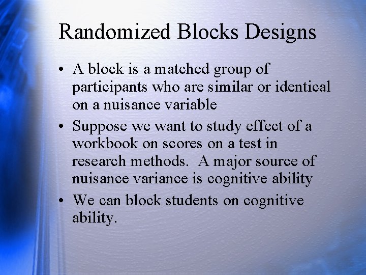
Randomized Blocks Designs • A block is a matched group of participants who are similar or identical on a nuisance variable • Suppose we want to study effect of a workbook on scores on a test in research methods. A major source of nuisance variance is cognitive ability • We can block students on cognitive ability.

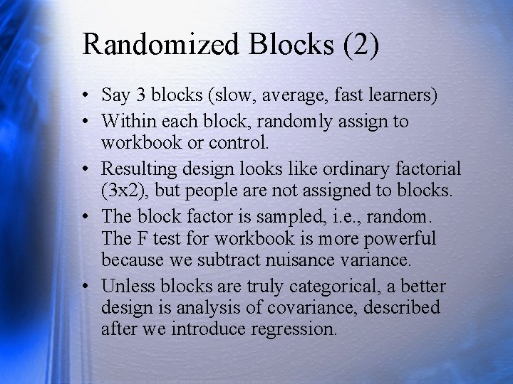
Randomized Blocks (2) • Say 3 blocks (slow, average, fast learners) • Within each block, randomly assign to workbook or control. • Resulting design looks like ordinary factorial (3 x 2), but people are not assigned to blocks. • The block factor is sampled, i. e. , random. The F test for workbook is more powerful because we subtract nuisance variance. • Unless blocks are truly categorical, a better design is analysis of covariance, described after we introduce regression.

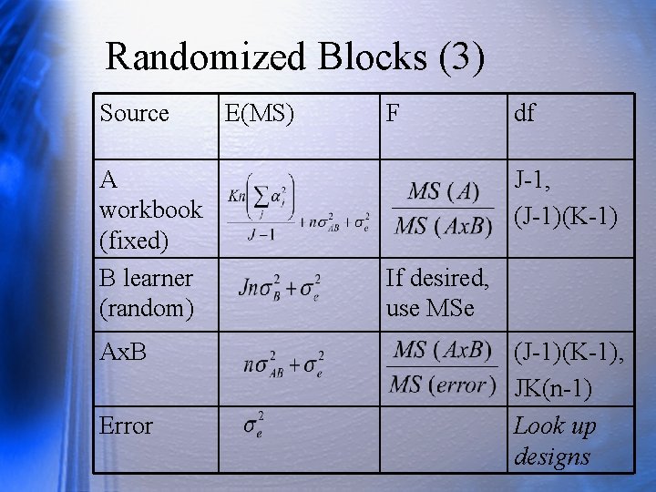
Randomized Blocks (3) Source A workbook (fixed) B learner (random) Ax. B Error E(MS) F df J-1, (J-1)(K-1) If desired, use MSe (J-1)(K-1), JK(n-1) Look up designs

Review q. Describe a concrete example of a randomized block design. You should have 1 factor as the blocking factor and one other factor as the factor of main interest. q. Describe a study in which Depression is a blocking factor.

Repeated Measures Designs • In a repeated measures design, participants appear in more than one cell. – Painfree study – Sports instruction • Commonly used in psychology

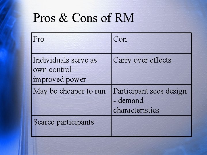
Pros & Cons of RM Pro Con Individuals serve as Carry over effects own control – improved power May be cheaper to run Participant sees design - demand characteristics Scarce participants

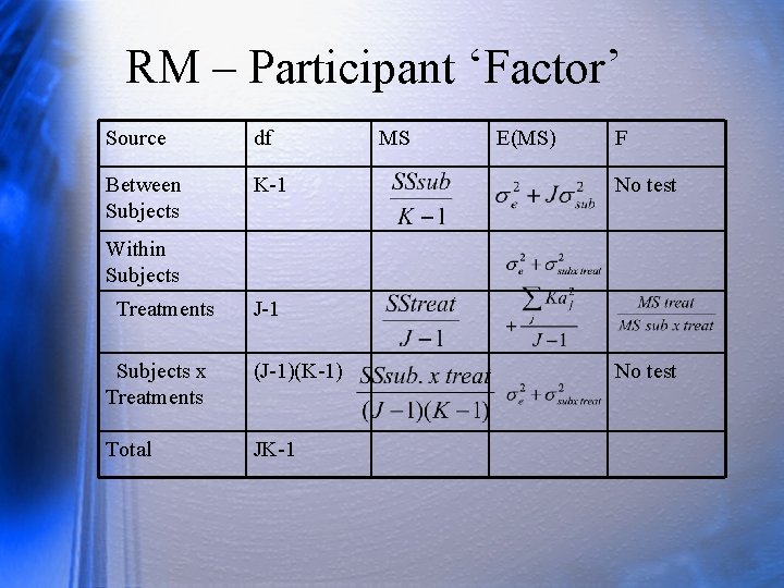
RM – Participant ‘Factor’ Source df Between Subjects K-1 MS E(MS) F No test Within Subjects Treatments J-1 Subjects x Treatments (J-1)(K-1) Total JK-1 No test

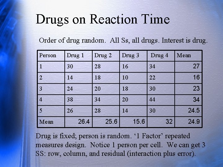
Drugs on Reaction Time Order of drug random. All Ss, all drugs. Interest is drug. Person Drug 1 Drug 2 Drug 3 Drug 4 1 30 28 16 34 27 2 14 18 10 22 16 3 24 20 18 30 23 4 38 34 20 44 34 5 26 28 14 30 24. 5 Mean 26. 4 25. 6 15. 6 32 Mean 24. 9 Drug is fixed; person is random. ‘ 1 Factor’ repeated measures design. Notice 1 person per cell. We can get 3 SS: row, column, and residual (interaction plus error).

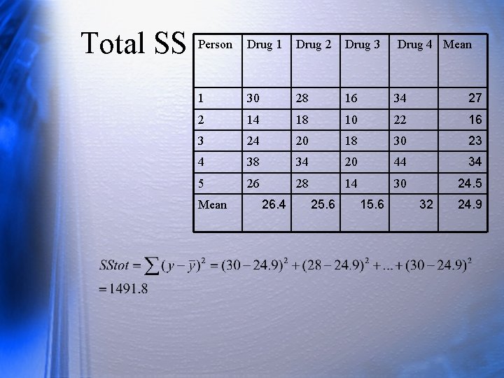
Total SS Person Drug 1 Drug 2 Drug 3 Drug 4 Mean 1 30 28 16 34 27 2 14 18 10 22 16 3 24 20 18 30 23 4 38 34 20 44 34 5 26 28 14 30 24. 5 Mean 26. 4 25. 6 15. 6 32 24. 9

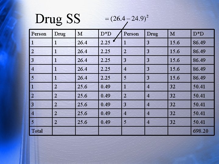
Drug SS Person Drug M D*D 1 1 26. 4 2. 25 1 3 15. 6 86. 49 2 1 26. 4 2. 25 2 3 15. 6 86. 49 3 1 26. 4 2. 25 3 3 15. 6 86. 49 4 1 26. 4 2. 25 4 3 15. 6 86. 49 5 1 26. 4 2. 25 5 3 15. 6 86. 49 1 2 25. 6 0. 49 1 4 32 50. 41 2 2 25. 6 0. 49 2 4 32 50. 41 3 2 25. 6 0. 49 3 4 32 50. 41 4 2 25. 6 0. 49 4 4 32 50. 41 5 2 25. 6 0. 49 5 4 32 50. 41 Total 698. 20

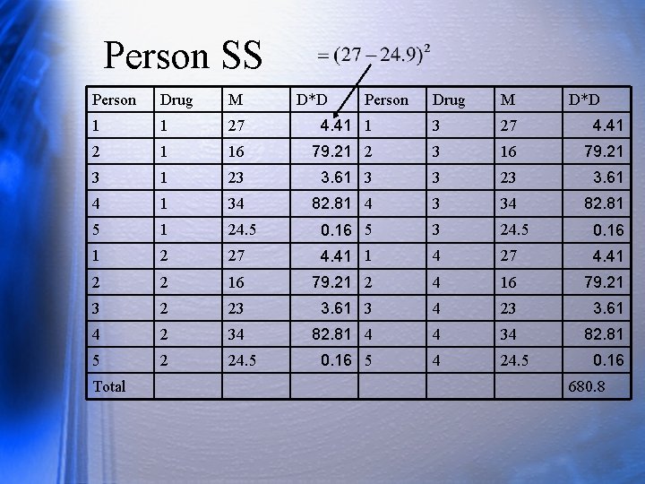
Person SS Person Drug M 1 1 27 2 1 3 Drug M 4. 41 1 3 27 4. 41 16 79. 21 2 3 16 79. 21 1 23 3. 61 3 3 23 3. 61 4 1 34 82. 81 4 3 34 82. 81 5 1 24. 5 0. 16 5 3 24. 5 0. 16 1 2 27 4. 41 1 4 27 4. 41 2 2 16 79. 21 2 4 16 79. 21 3 2 23 3. 61 3 4 23 3. 61 4 2 34 82. 81 4 4 34 82. 81 5 2 24. 5 0. 16 5 4 24. 5 Total D*D Person D*D 0. 16 680. 8

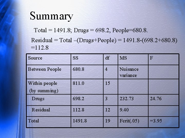
Summary Total = 1491. 8; Drugs = 698. 2, People=680. 8. Residual = Total –(Drugs+People) = 1491. 8 -(698. 2+680. 8) =112. 8 Source SS df MS Between People 680. 8 4 Nuisance variance Within people (by summing) 811. 0 15 Drugs 698. 2 3 232. 73 Residual 112. 8 12 9. 40 1491. 8 19 Fcrit(. 05) Total F 24. 76 =3. 95

SAS Run the same problem using SAS.

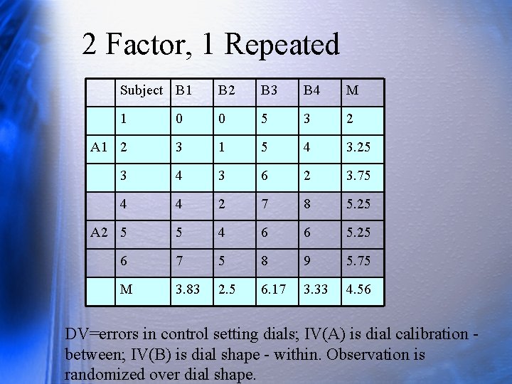
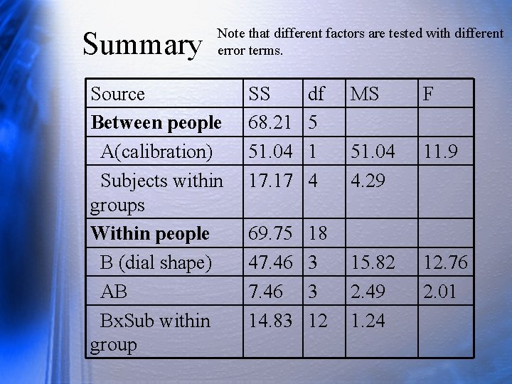
2 Factor, 1 Repeated Subject B 1 B 2 B 3 B 4 M 1 0 0 5 3 2 A 1 2 3 1 5 4 3. 25 3 4 3 6 2 3. 75 4 4 2 7 8 5. 25 A 2 5 5 4 6 6 5. 25 6 7 5 8 9 5. 75 M 3. 83 2. 5 6. 17 3. 33 4. 56 DV=errors in control setting dials; IV(A) is dial calibration between; IV(B) is dial shape - within. Observation is randomized over dial shape.

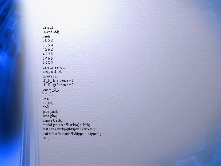
data d 1; input i 1 -i 4; cards; 0053 3154 4362 4278 5466 7589 data d 2; set d 1; array z i 1 -i 4; do over z; if _N_ le 3 then a =1; if _N_ gt 3 then a =2; sub = _N_; b = _I_; y=z; output; end; proc print; proc glm; class a b sub; model y = a b a*b sub(a) sub*b; test h=a e=sub(a)/htype=1 etype=1; test h=b a*b e=sub*b/htype=1 etype=1; run;

Summary Note that different factors are tested with different error terms. Source Between people A(calibration) Subjects within groups Within people B (dial shape) AB Bx. Sub within group SS 68. 21 51. 04 17. 17 df 5 1 4 69. 75 47. 46 14. 83 18 3 3 12 MS F 51. 04 4. 29 11. 9 15. 82 2. 49 1. 24 12. 76 2. 01

SAS & Post Hoc Tests Run the same problem using SAS. The SAS default is to use what ever is residual as denominator of F test. You can use this to your advantage or else over-ride it to produce specific F tests of your desire. If you use the default error term, be sure you know what it is. Post hoc tests with repeated measures are tricky. You have to use the proper error term for each test. The error term changes depending on what you are testing. Be sure to look up the right error term.

Assumptions of RM Orthogonal ANOVA assumes homogeneity of error variance within cells. IVs are independent. With repeated measures, we introduce covariance (correlation) across cells. For example, the correlation of scores across subjects 1 -3 for the first two calibrations is. 89. Repeated measures designs make assumptions about the homogeneity of covariance matrices across conditions for the F test to work properly. If the assumptions are not met, you have problems and may need to make adjustments. You can avoid these assumptions by using multivariate techniques (MANOVA) to analyze your data. I suggest you do so. If you use ANOVA, you need to look up your design to get the right F tests and check on the assumptions.

Review q How is a repeated measures design different from a totally between subjects design in the collection of the data? q How does the significance testing change from the totally between to a design to one in which one or more factors are repeated measures (just the general idea, you don’t need to show actual F ratios or computations)? q Describe one argument for using repeated measures designs and one argument against using such designs (or describe when you would and would not want to use repeated measures).