RADON TRANSFORM A small introduction to RT its

RADON TRANSFORM A small introduction to RT, its inversion and applications Jaromír Brum Kukal, 2009

Johann Karl August Radon • Born in Děčín (Austrian monarchy, now North Bohemia, CZ) in 1887 • Austrian mathematician living in Vienna • Discover the transform and its inversion in 1917 as pure theoretical result • No practical applications during his life • Died in 1956 in Vienna

Actual applications of inverse Radon transform • CT – Computer Tomography • MRI – Magnetic Resonance Imaging • PET – Positron Emission Tomography • SPECT – Single Photon Emission Computer Tomography

Geometry of 2 D Radon transform • Input space coordinates x, y • Input function f(x, y) • Output space coordinates a, s • Output function F(a, s)

Theory of pure RT and IRT Radon transform Inverse Radon transform

Full circle in RT

Shifted full circle in RT

Empty circle in RT

Shifted empty circle in RT

Thin stick in RT

Shifted thin stick in RT

Full triangle in RT

Shifted full triangle in RT

Full square in RT

Shifted full square in RT

Empty square in RT

Shifted empty square in RT

| x |2/3 + | y |2/3 ≤ 1 in RT

| x |3/2 + | y |3/2 ≤ 1 in RT

| x |2 + | y |2 ≤ 1 in RT

| x |6 + | y |6 ≤ 1 in RT

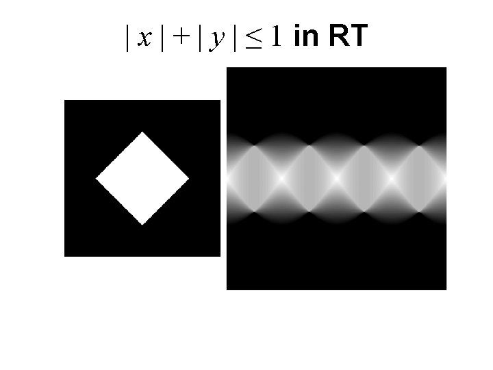
| x |n + | y |n ≤ 1 for n in RT

2 D Gaussian in RT

Shifted 2 D Gaussian in RT

Six 2 D Gaussians in RT

Smooth elliptic object in RT

Radon transform applications Natural transform as result of measurement: • Gamma ray decay from local density map • Extinction from local concentration map • Total radioactivity from local concentration map • Total echo from local nuclei concentration map • 3 D reality is investigated via 2 D slices Artificial realization: • Noise – RT – noise – IRT simulations • Image decryption as a fun • TSR invariant recognition of objects

Radon transform properties • Image of any f + g is F + G • Image of cf is c. F for any real c • Rotation of f causes translation of F in α • Scaling of f in (x, y) causes scaling of F in s • Image of a point (2 D Dirac function) is sine wave line • Image of n points is a set of n sine wave lines • Image of a line is a point (2 D Dirac function) • Image of polygon contour is a point set

Radon transform realization Space domain: • Pixel splitting into four subpixels • 2 D interpolation in space domain • 1 D numeric integration along lines Frequency domain: • 2 D FFT of original • Resampling to polar coordinates • 2 D interpolation in frequency domain • Inverse 2 D FFT brings result

Inverse transform realization Filtered back projection in space domain: • 1 D HF filtering of 2 D original along s • Additional 1 D LF filtering along s • 2 D interpolation in space domain • 1 D integration along lines brings result Frequency domain: • 2 D FFT of original • Resampling to rectangular coordinates • 2 D interpolation in frequency domain • 2 D LF filtering in frequency domain • Inverse 2 D FFT brings result

RT and IRT in Matlab • Original as a square matrix D (2 n 2 n) of nonnegative numbers • Vector of angles alpha • Basic range alpha = 0: 179 • Digital range is better alpha = (0: 2^N -1)*180/2^N • Extended range alpha = 0: 359 • Output matrix R of nonnegative numbers • Angles alpha generates columns of R R = radon(D, alpha); D = iradon(R, alpha, metint, metfil);

Reconstruction from 32 angles

Reconstruction from 64 angles

Reconstruction from 96 angles

Reconstruction from 128 angles

Reconstruction from 180 angles

Reconstruction from 256 angles

Reconstruction from 360 angles

Reconstruction from 512 angles