Radiowave Propagation Mechanisms A Introduction to Radiowave propagation

Radiowave Propagation Mechanisms A. Introduction to Radiowave propagation B. Free Space Propagation Model CO-2 COI-1

Introduction • Wired channels are stationary and predictable. • Radio channels are extremely random, timevarying and have complex models. • Transmission path between Tx and Rx can vary in complexity. üLine of Sight (LOS) üNon line of Sight (NLOS)

Radio wave Propagation • Most of the time, radio waves are not quite in free space. • Terrestrial propagation modes include: – Line-of-sight propagation – Space-wave propagation – Ground waves – Sky waves

Radio wave Propagation Ionosphere (80 - 720 km) Sky wave Mesosphere (50 - 80 km) Stratosphere (12 - 50 km) Space wave er itt m s n a Tr Ground wave Rece iver Earth Troposphere (0 - 12 km) 6

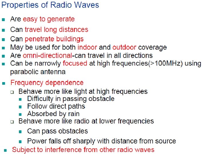
Radio Frequency Bands Classification Band Initials Frequency Range Extremely low ELF < 300 Hz Infra low ILF 300 Hz - 3 k. Hz Very low VLF 3 k. Hz - 30 k. Hz Low LF 30 k. Hz - 300 k. Hz Medium MF 300 k. Hz - 3 MHz Ground/Sky wave High HF 3 MHz - 30 MHz Sky wave Very high VHF 30 MHz - 300 MHz Ultra high UHF 300 MHz - 3 GHz Super high SHF 3 GHz - 30 GHz Extremely high EHF 30 GHz - 300 GHz Tremendously high THF 300 GHz - 3000 GHz Characteristics Ground wave Space wave

Radio Wave Components Wave component Comments Direct wave Free-space propagation Reflected wave Reflection from passive antenna, ground, wall, object, ionosphere <~100 MHz, etc. Refracted wave Standard, Sub-, and Super-refraction, ducting, ionized layer refraction <~100 MHz Diffracted wave Ground-, mountain-, spherical earthdiffraction <~5 GHz Surface wave <~30 MHz Scatter wave Troposcatter wave, precipitation-scatter wave, ionized-layer scatter wave

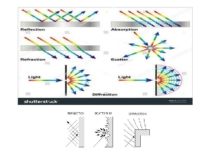
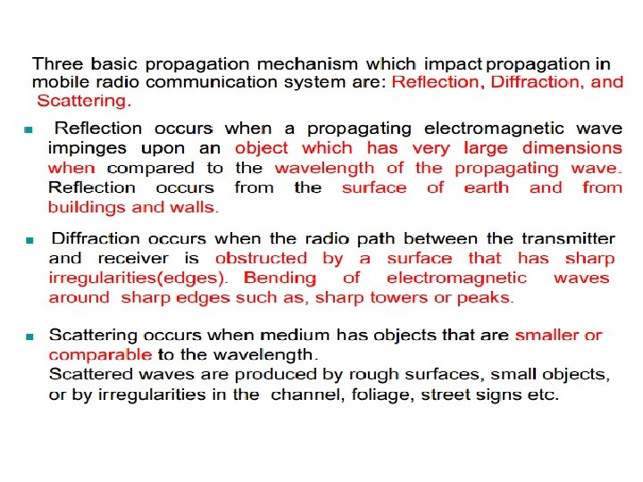
Radiowave Propagation Mechanisms • Absorption − Conversion of the transmitted EM energy into another form, usually thermal −E. g. , Signal attenuation due to precipitations (rain, snow, sand) and atmospheric gases • Refraction −Redirection of a wave-front passing through a medium having a refractive index that is a continuous function of position or through a boundary between two dissimilar media. −e. g. , A graded-index optical fiber, or Earth’s atmosphere • Reflection – Propagation wave impinges on an object which is large as compared to wavelength - e. g. , the surface of the Earth, buildings, walls, etc.

Reflection Corner reflector Parabolic reflector Diffuse Reflection

Refraction • Results in the bending of radio waves • Snell’s Law governs the behavior

Propagation Mechanisms • Diffraction – Radio path between transmitter and receiver obstructed by surface with sharp irregular edges – Waves bend around the obstacle, even when LOS (line of sight) does not exist • Scattering – Objects smaller than the wavelength of the propagation wave - e. g. foliage, street signs, lamp posts

Diffraction • As a result, waves can appear to “go around corners” • Diffraction is more apparent when the object has sharp edges

Scattering • Tropospheric Scatter - makes use of the scattering of radio waves in the troposphere to propagate signals in the 250 MHz – 5 GHz range

Radio Wave Propagation Effects

Radio Wave Propagation Effects Building Direct Signal Reflected Signal hb Diffracted Signal hm d Transmitter Receiver

Propagation Models q Large Scale Propagation Model: Predicting the average received signal strength at a given distance from Tx. q Small Scale or Fading Models: Variability of signal strength in the close proximity of Tx

Small-scale and Large-scale fading Small-scale fading Large-scale variations

Propagation Models *Mechanisms involved in radio wave propagation : –Reflection –Diffraction –Scattering *Most Cellular Radio systems operate in Urban areas: –No direct line-of-sight –high-rise buildings causes severe diffraction loss –multipath fading due to different paths of varying lengths

Propagation Models Large-scale propagation models: ü Predict the mean signal strength for an arbitrary transmitter-receiver (T-R) separation distance. ü Estimate radio coverage of a transmitter. ü Separation distances (several 100’s to 1000’s meters). ü Local average received power is predicted (measurement track of 5 λ to 40 λ ).

Propagation Models Small-scale or fading models: ü Characterize RAPID fluctuations of the received signal strength over very short travel distance (a few wavelengths) ü Short time duration (on the order of seconds) ü Sum of many contributions from different directions with different phases ü Random phases cause the sum varying widely. (ex: Rayleigh fading distribution)

Free Space Propagation Model Signal strength (log) It predicts received signal strength when T and R have a clear (unobstructed) LOS path between them. –Satellite communication –Microwave line-of-sight radio link Free space Open area (LOS) Urban Suburban Distance (log)

Basic Transmission Theory Isotropic Source Distance R Pt Watts Surface Area of sphere = 4 p. R 2 encloses Pt. Power Flux Density: W/m 2

Basic Transmission Theory For Isotropic source, the Flux density in the antenna sight direction is: Received power:

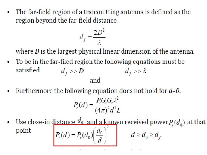
Received Power Effective Isotropic Radiated Power (EIRP) Path loss/ Free Space Loss

Free Space Propagation Model Free space Power received by a Receiver antenna separated from a radiating Transmitter antenna by a distance ‘d’ is given by Friis free space equation;

Path Loss

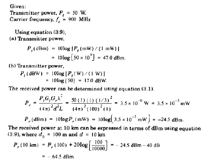
• d. Bm and d. BW units are used • Pr in d. Bm is: