Radionuclide dispersion modelling Radiation Protection of the Environment
")


:")

, mixing")


 or soil")

 ¥ Mixing")


 Some")
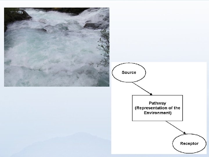
 Lz = distance to achieve full vertical mixing (=7 D) Estuaries")
 •")

- Slides: 20
Radionuclide dispersion modelling Radiation Protection of the Environment (Environment Agency Course, July 2015)
By the end of the presentation and practical you should…. ¥ Understand the purpose of dispersion models ¥ Know the origin of the dispersion models used in ERICA ¥ Be able to use some of the basic dispersion models provided in ERICA
What happens if do not have media concentration? ¥ ¥ ¥ Need method of predicting from release rates If have dispersion model can run and input predictions If not then ERICA has some screening level models built-in to enable this in Tiers 1 and 2
Taken from IAEA SRS Publication 19 ¥ Designed to minimise underprediction (conservative generic assessment): ‘Under no circumstances would doses be underestimated by more than a factor of ten. ’ ¥ A default discharge period of 30 y is assumed (estimates doses for the 30 th year of discharge) ¥ Models - atmospheric, freshwater (lakes and rivers) and coastal water models available
Taken from IAEA SRS Publication 19 ¥ ¥ ¥ Designed to minimise underprediction (conservative generic assessment): ‘Under no circumstances would doses be underestimated by more than a factor of ten. ’ SRS-19 is linked to ERICA help file A default discharge period of 30 y is assumed (estimates doses for the 30 th year of discharge) Models - atmospheric, freshwater (lakes and rivers) and coastal water models available
Atmospheric dispersion ¥ ¥ ¥ Simple atmospheric dispersion model incorporating downwind transport (advection), mixing (turbulent diffusion) and effects of buildings For continuous, long-term release (not accidents) Gaussian plume model (=normal distribution in vertical and lateral axis) ¥ ¥ Not applicable >20 km from release in ERICA assume 20 km if >20 km ¥ Assumes a predominant wind direction and neutral stability class (=doesn’t enhance or inhibit turbulence) ¥ If you (really) want all the equations – see SRS-19
Atmospheric dispersion
Atmospheric dispersion Importance of Release Height Effective stack height
Conditions for the plume
Conditions for the plume
Output ¥ Radionuclide activity concentrations in air (C, H, S & P) or soil (everything else)
Surface water dispersion ¥ Freshwater ¥ ¥ ¥ Marine ¥ ¥ ¥ Small lake (< 400 km 2) Large lake (≥ 400 km 2) Estuarine River Coastal Estuarine No model for open ocean waters
Processes and assumptions ¥ Processes included: ¥ Flow downstream as transport (advection) ¥ Mixing processes (turbulent dispersion) ¥ Concentration in sediment estimated from ERICA Kd at receptor (equilibrium) ¥ No loss to sediment between source and receptor ¥ Half-life drives difference between RN in water ¥ River flow conditions – 30 y low assumed
Small lakes and reservoirs ¥ ¥ Assumes a homogeneous concentration throughout the water body Expected life time of facility is required as input
Large Lake ¥ >400 km 2 ‘. . as a rough rule a lake can be considered to be large when the opposite side of the lake is not visible to a person standing on a 30 m high shore. ’
Large Lake Some restrictions related to short receptor discharge point distances (mixing zone) Some restrictions related to length discharge pipe and angle to shoreline receptor Estimates concentration along shoreline Estimates concentration along plume centre line
Rivers (& Estuaries) Lz = distance to achieve full vertical mixing (=7 D) Estuaries model similar to rivers • Some tidal parameters used
Some restrictionswaters related to: Coastal • short receptor discharge point distances (mixing zone) • length discharge pipe and angle to shoreline receptor Dispersion along the coast • Shoreline or ‘in sea’ receptors For 10’s km (not >100 km)
Summary limitations of IAEA SRS 19 ¥ Simple environmental and dosimetric models as well as sets of necessary default data: ¥ ¥ ¥ Simplest, linear compartment models Simple screening approach (robust but conservative) Short source-receptor distances Equilibrium between liquid and solid phases - Kd More complex / higher tier assessments: ¥ ¥ Aerial model includes only one wind direction Coastal dispersion model not intended for open waters e. g. oil/gas marine platform discharges Surface water models assume geometry (e. g. river crosssection) & flow characteristics (e. g. velocity, water depth) which do not change significantly with distance / time End of pipe mixing zones require hydrodynamic models