Radio Frequency TOF Distance Measurement for LowCost Wireless

Radio Frequency TOF Distance Measurement for Low-Cost Wireless Sensor Localization Steven Lanzisera, David Zats and Kristofer S. J. Pister

Introduction 1. • Paper was published in 2010 • Localization is a hot topic – Creating location-aware sensor networks – Enabling mobile phones to host a lot of new applications • Requirements – Low-cost / low energy consumption is crucial – If we require a certain accuracy – we have to deal with measurement errors

Introduction 2. • Methods of localization – Acustic (Beep, we have seen it) – RF techniques (no GPS) – GPS • The paper proposes an RF solution – Low cost / narrowband – No time-syncronization required – No base-station required – Approaches the Cramér-Rao bound in noisy environment – Accuracy – only in the order of a few meters (!)

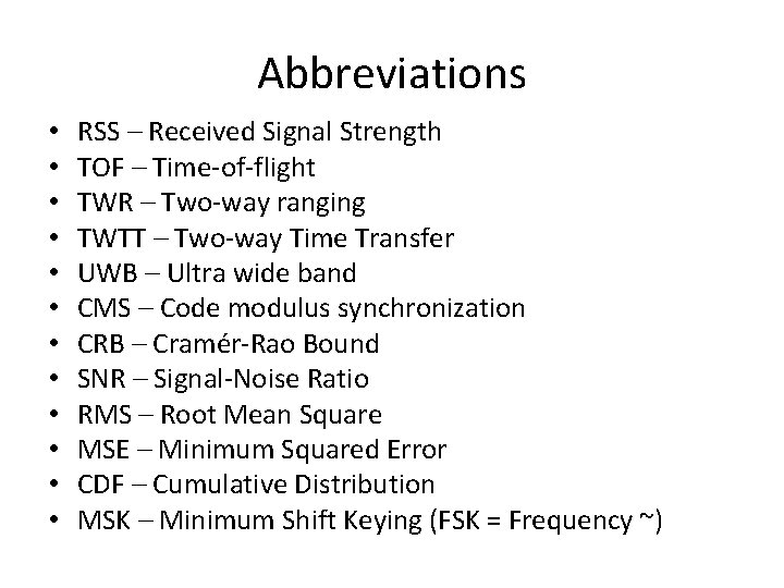
Abbreviations • • • RSS – Received Signal Strength TOF – Time-of-flight TWR – Two-way ranging TWTT – Two-way Time Transfer UWB – Ultra wide band CMS – Code modulus synchronization CRB – Cramér-Rao Bound SNR – Signal-Noise Ratio RMS – Root Mean Square MSE – Minimum Squared Error CDF – Cumulative Distribution MSK – Minimum Shift Keying (FSK = Frequency ~)

Localization problem • Localization consists of two parts – Measure relationships between nodes – Using this information to determine position of nodes • Received Signal Strength – Well-studied method – Determines range based on signal strength – Very inaccurate

Alternatives • Using Ultra Wide Band ranging – UWB receivers are very complex and expensive • Narrowband solutions – They usually require time synchronization, that adds complexity again • A low cost – simple technology is needed with meter-level accuracy

The presented system • Two-way ranging system • CMS (Code modulus synchronization) – No time-sync required – Online measurement – Offline range extraction • Works well in noise-limited environment • Mitigates the effects of multipath propagation – Idea: take measurements on multiple frequencies • Approaches the Cramér-Rao bound • Room-level accuracy satisfied (~1 -3 m)

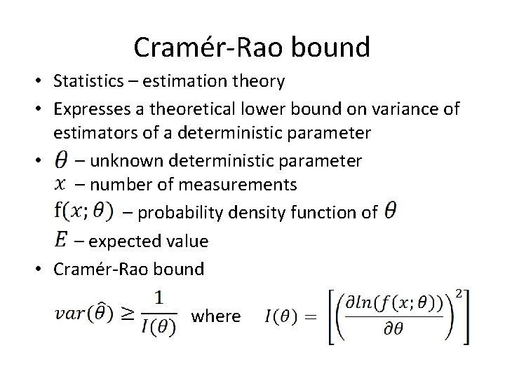
Cramér-Rao bound • Statistics – estimation theory • Expresses a theoretical lower bound on variance of estimators of a deterministic parameter • – unknown deterministic parameter – number of measurements – probability density function of – expected value • Cramér-Rao bound where

Test-implementation • Commercially available accessories • 2. 4 GHz radio – Frequency Shift Keying • IEEE 802. 15. 4 – Standard which specifies physical layer and media access control for low-rate wireless PANs – Zigbee, Mi. Wi. . . etc. • FPGA • Overall accuracy: 1 m outdoor / 1 -3 m indoor

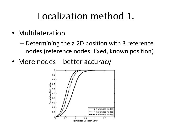
Localization method 1. • Multilateration – Determining the a 2 D position with 3 reference nodes (reference nodes: fixed, known position) • More nodes – better accuracy

Localization method 2. • More reference nodes should be used than strictly necessary • The geometry of the ref. nodes is important – Collinear references do not work • This area is highly understood, the more important part is determining the position from erroneous measurements

Range estimation methods • RSS – constructive and destructive interference make it unsuitably inaccurate • Time-of-Flight methods – Speed of light = 299, 792, 458 m/s – 1 meter range accuracy = 3 ns time resolution – Low-cost devices provide the sampling resolution as their clock frequency ~50 ns – Cost, complexity and terrestrial environment (in comparison with GPS) make TOF ranging unsuitable

Types of errors to consider • • Clock synchronization Noise Errors of samping artifacts Multipath channel effects

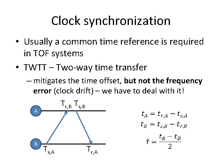
Clock synchronization • Usually a common time reference is required in TOF systems • TWTT – Two-way time transfer – mitigates the time offset, but not the frequency error (clock drift) – we have to deal with it! Tr, B Ts, B A B Ts, A Tr, A

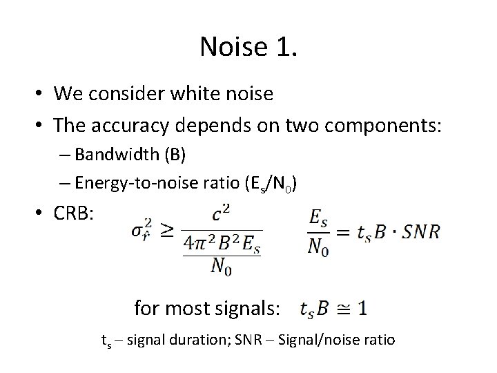
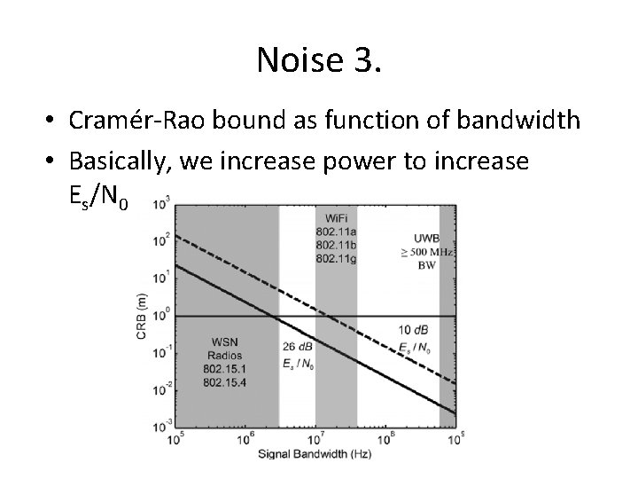
Noise 1. • We consider white noise • The accuracy depends on two components: – Bandwidth (B) – Energy-to-noise ratio (Es/N 0) • CRB: for most signals: ts – signal duration; SNR – Signal/noise ratio

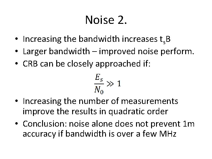
Noise 2. • Increasing the bandwidth increases ts. B • Larger bandwidth – improved noise perform. • CRB can be closely approached if: • Increasing the number of measurements improve the results in quadratic order • Conclusion: noise alone does not prevent 1 m accuracy if bandwidth is over a few MHz

Noise 3. • Cramér-Rao bound as function of bandwidth • Basically, we increase power to increase Es/N 0

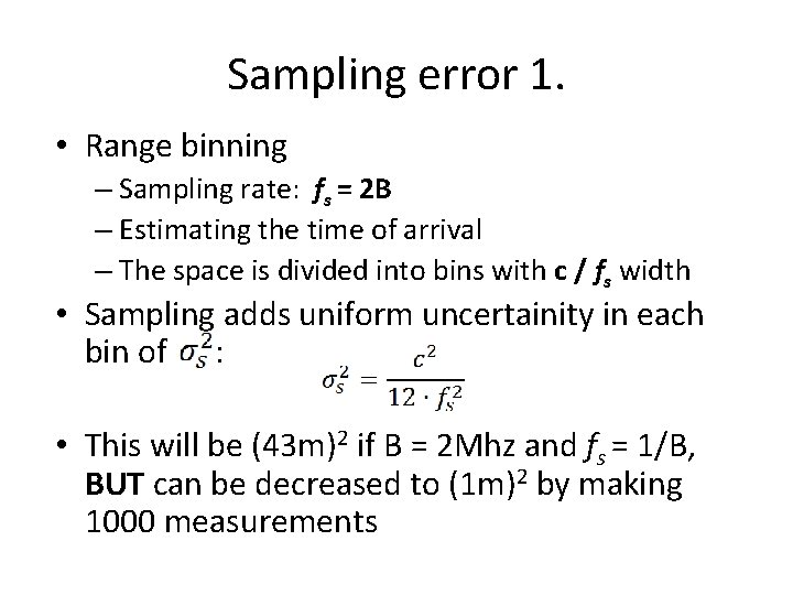
Sampling error 1. • Range binning – Sampling rate: fs = 2 B – Estimating the time of arrival – The space is divided into bins with c / fs width • Sampling adds uniform uncertainity in each bin of : • This will be (43 m)2 if B = 2 Mhz and fs = 1/B, BUT can be decreased to (1 m)2 by making 1000 measurements

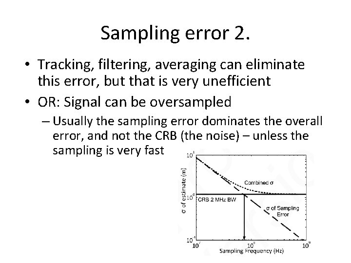
Sampling error 2. • Tracking, filtering, averaging can eliminate this error, but that is very unefficient • OR: Signal can be oversampled – Usually the sampling error dominates the overall error, and not the CRB (the noise) – unless the sampling is very fast

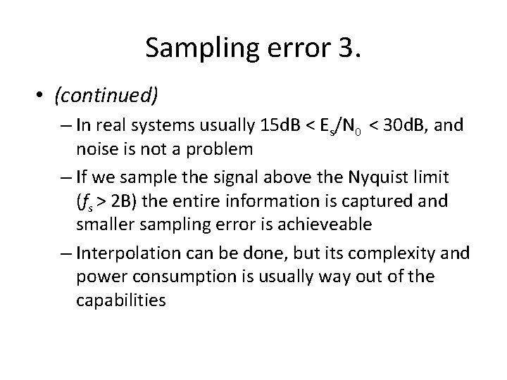
Sampling error 3. • (continued) – In real systems usually 15 d. B < Es/N 0 < 30 d. B, and noise is not a problem – If we sample the signal above the Nyquist limit (fs > 2 B) the entire information is captured and smaller sampling error is achieveable – Interpolation can be done, but its complexity and power consumption is usually way out of the capabilities

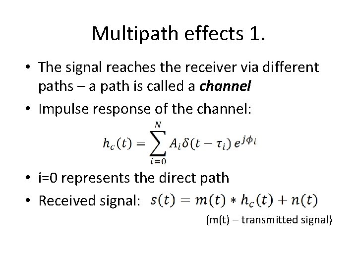
Multipath effects 1. • The signal reaches the receiver via different paths – a path is called a channel • Impulse response of the channel: • i=0 represents the direct path • Received signal: (m(t) – transmitted signal)

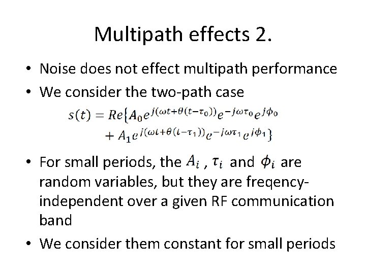
Multipath effects 2. • Noise does not effect multipath performance • We consider the two-path case • For small periods, the , and are random variables, but they are freqencyindependent over a given RF communication band • We consider them constant for small periods

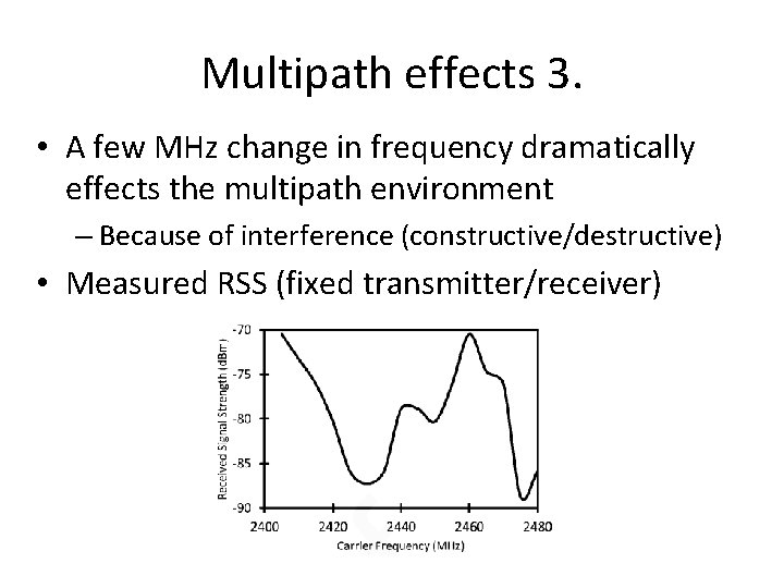
Multipath effects 3. • A few MHz change in frequency dramatically effects the multipath environment – Because of interference (constructive/destructive) • Measured RSS (fixed transmitter/receiver)

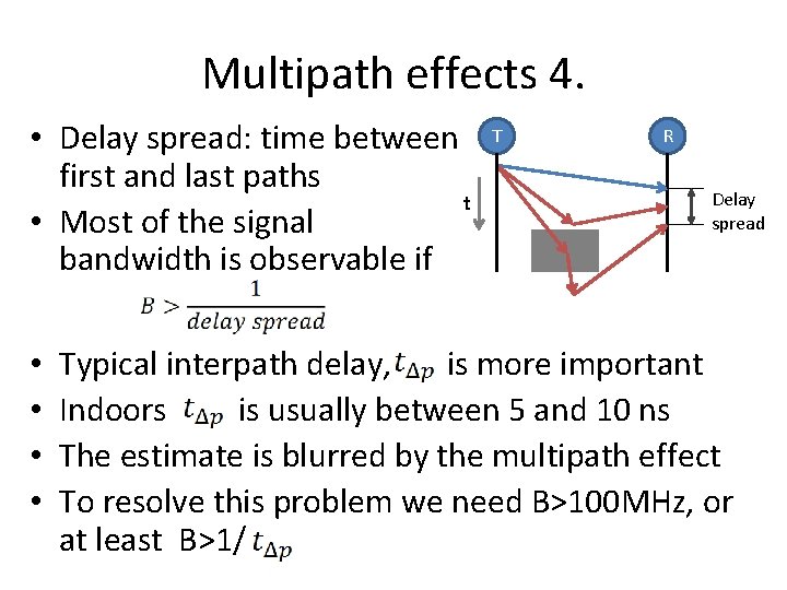
Multipath effects 4. • Delay spread: time between first and last paths t • Most of the signal bandwidth is observable if • • T R Delay spread Typical interpath delay, is more important Indoors is usually between 5 and 10 ns The estimate is blurred by the multipath effect To resolve this problem we need B>100 MHz, or at least B>1/

Multipath effects 5. • Possible solutions to mitigate multipath effects: – Increase bandwidth – Estimating channel impulse response – Multipath bias reduction • The first two are well-studied • Using devices with larger bandwidth (UWB) is expensive and they consume to much power • The achieveable accuracy appears to be around 30 m with the second method – not sufficient

The solution

Ranging error mitigation • The paper presents two new methods to mitigate all the errors – Code modulus synchonrization • Combats sampling effects and poor time syncronization – Frequency diverse range estimation • Improves range estimation accuracy

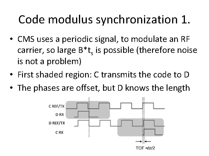
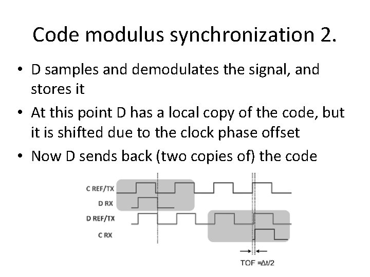
Code modulus synchronization 1. • CMS uses a periodic signal, to modulate an RF carrier, so large B*ts is possible (therefore noise is not a problem) • First shaded region: C transmits the code to D • The phases are offset, but D knows the length

Code modulus synchronization 2. • D samples and demodulates the signal, and stores it • At this point D has a local copy of the code, but it is shifted due to the clock phase offset • Now D sends back (two copies of) the code

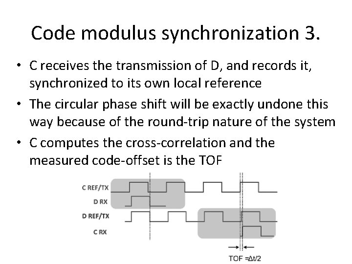
Code modulus synchronization 3. • C receives the transmission of D, and records it, synchronized to its own local reference • The circular phase shift will be exactly undone this way because of the round-trip nature of the system • C computes the cross-correlation and the measured code-offset is the TOF

Code modulus synchronization 4. • The received code can be interpolated to improve resolution up to the noise limit • The system approaches the CRB even with a single measurement • Multiple measurements can be averaged – this helps achieving good noise-performance • Correlation and code-offset estimation can be done offline after the RT part has ended

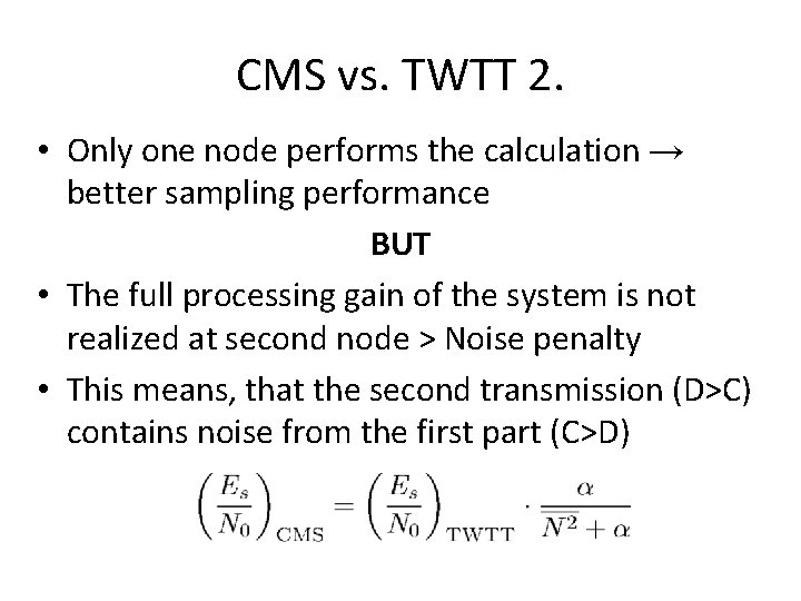
CMS vs. TWTT 1. • CMS vs. TWTT – Only one node performs the calculation → better sampling performance BUT – The full processing gain of the system is not realized at second node → Noise penalty – This means, that the second transmission (D→C) contains noise from the first part (C→D)

CMS vs. TWTT 2. • Only one node performs the calculation → better sampling performance BUT • The full processing gain of the system is not realized at second node > Noise penalty • This means, that the second transmission (D>C) contains noise from the first part (C>D)

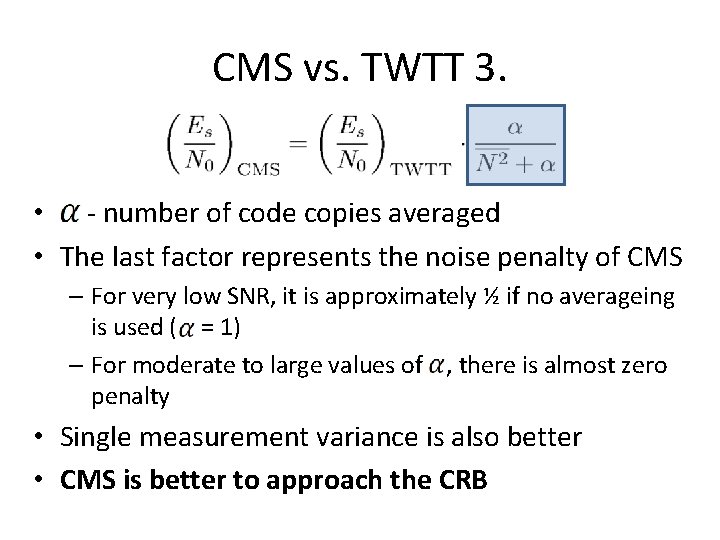
CMS vs. TWTT 3. • - number of code copies averaged • The last factor represents the noise penalty of CMS – For very low SNR, it is approximately ½ if no averageing is used ( = 1) – For moderate to large values of , there is almost zero penalty • Single measurement variance is also better • CMS is better to approach the CRB

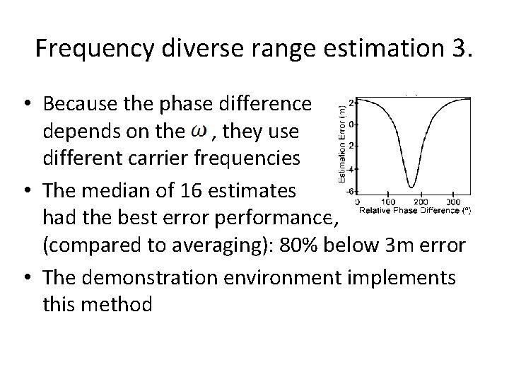
Frequency diverse range estimation 1. • Mitigates the multipath effect • Takes measurements on several carrier frequences • The problem: – Signal comes via two paths: one direct, more reflected – There is a delay and phase difference between them – Only the phase depends on the actual value – IEEE 802. 15. 4 uses MSK, a version of FSK – When changes to , the signal from the second path have not arrived yet

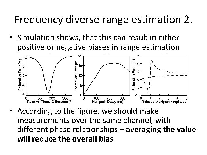
Frequency diverse range estimation 2. • Simulation shows, that this can result in either positive or negative biases in range estimation • According to the figure, we should make measurements over the same channel, with different phase relationships – averaging the value will reduce the overall bias

Frequency diverse range estimation 3. • Because the phase difference depends on the , they use different carrier frequencies • The median of 16 estimates had the best error performance, (compared to averaging): 80% below 3 m error • The demonstration environment implements this method

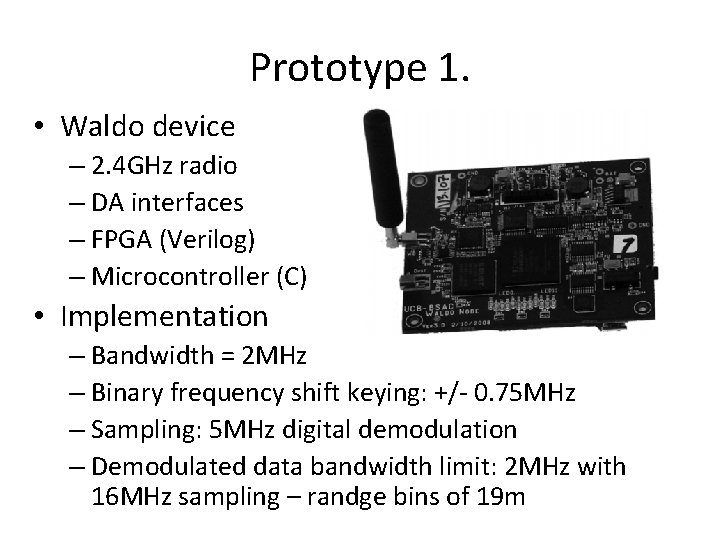
Prototype 1. • Waldo device – 2. 4 GHz radio – DA interfaces – FPGA (Verilog) – Microcontroller (C) • Implementation – Bandwidth = 2 MHz – Binary frequency shift keying: +/- 0. 75 MHz – Sampling: 5 MHz digital demodulation – Demodulated data bandwidth limit: 2 MHz with 16 MHz sampling – randge bins of 19 m

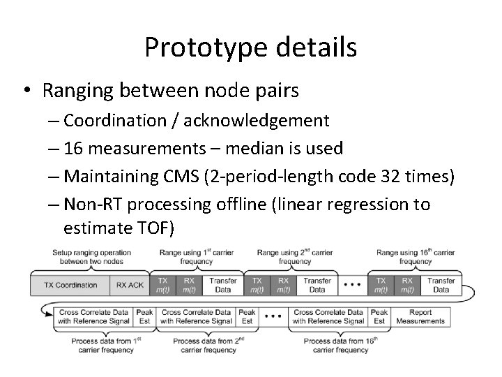
Prototype details • Ranging between node pairs – Coordination / acknowledgement – 16 measurements – median is used – Maintaining CMS (2 -period-length code 32 times) – Non-RT processing offline (linear regression to estimate TOF)

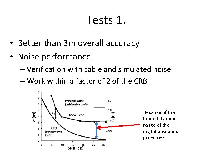
Tests 1. • Better than 3 m overall accuracy • Noise performance – Verification with cable and simulated noise – Work within a factor of 2 of the CRB Because of the limited dynamic range of the digital baseband processor

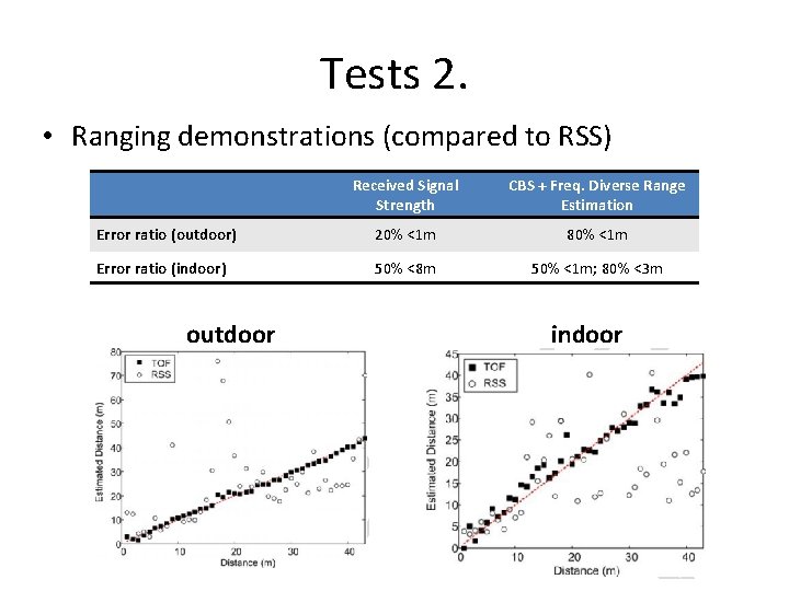
Tests 2. • Ranging demonstrations (compared to RSS) Received Signal Strength CBS + Freq. Diverse Range Estimation Error ratio (outdoor) 20% <1 m 80% <1 m Error ratio (indoor) 50% <8 m 50% <1 m; 80% <3 m outdoor indoor

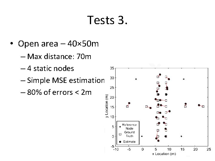
Tests 3. • Open area – 40× 50 m – Max distance: 70 m – 4 static nodes – Simple MSE estimation – 80% of errors < 2 m

Conclusion • CMS is a TWR method that approaches the CRB • Freq. diverse ranging estimation is a strategy that improves ranging in multipath environments • Overall accuracy: 1 m outdoors, 1 -3 m indoors • Where Es/N 0 is large, sampling error dominates the noise-induced error, but CMS avoids this • Easy implementation, low costs, no UWB device required

Thank you for you attention!