Radially symmetric 1 D Reference Earth Models JeffreysBullen

Radially symmetric (1 -D) Reference Earth Models • Jeffreys-Bullen Earth Model (JB) 1936 -1958 • Preliminary Reference Earth Model (PREM) Dziewonski & Anderson 1981 • IASPEI-91 Kennett & Engdahl (1991) • AK 135 Kennett et al (1995) • STW 105 ? Kustowski, Ekstrom, Dziewonski, 2008

Comparison of 1 -D Reference Models

Comparing Models Upper Mantle Structure

Travel-time tomography -- Uses observed travel time for many source-receiver combinations to reconstruct seismic velocity image -- Solves for the slowness sj = 1/vj of each block (node) -- Travel time for each observation is the sum of travel times in each block t = Lj sj -- The matrix equation for all the travel times is: ti = Lij sj -- Least Squares Solution: s = [LTL]-1 LTt -- Can be applied to traditional body wave or surface wave data

Regional Body Wave Tomography – Tonga Subduction Zone Raypaths Velocity Conder & Wiens [2006]

Full waveform inversion Compute complete synthetic seismograms by simulating wave propagation using finite elements (in this case, spectral element) Compute the misfit of the synthetics to the observed data Then perturb the velocity model to reduce the misfit We do this using an adjoint inversion Generally takes many iterations

Full Waveform Inversion

Adjoint tomography The misfit is propagated back in time (Adjoint wavefield) The interaction field is the product of the forward and adjoint wavefields The Event Kernel identifies all the regions that could have contributed to the misfit Tape et al, 2007

Example: Full Waveform Inversion of Antarctica

Downside of Adjoint Full Waveform Tomography • Computationally Expensive (~80, 000 CPU*hrs/iteration) • Difficult to determine uncertainties

Global 3 -D tomographic models parameterization Spherical Harmonic expansion Boxes Nodes Multi-scale (irregular volumes) Data: Surface waves (shallow) & body waves (deep) Sometimes: modes Voronoi Cells

Difficulties with seismic tomography Sources and Receivers Ray path density

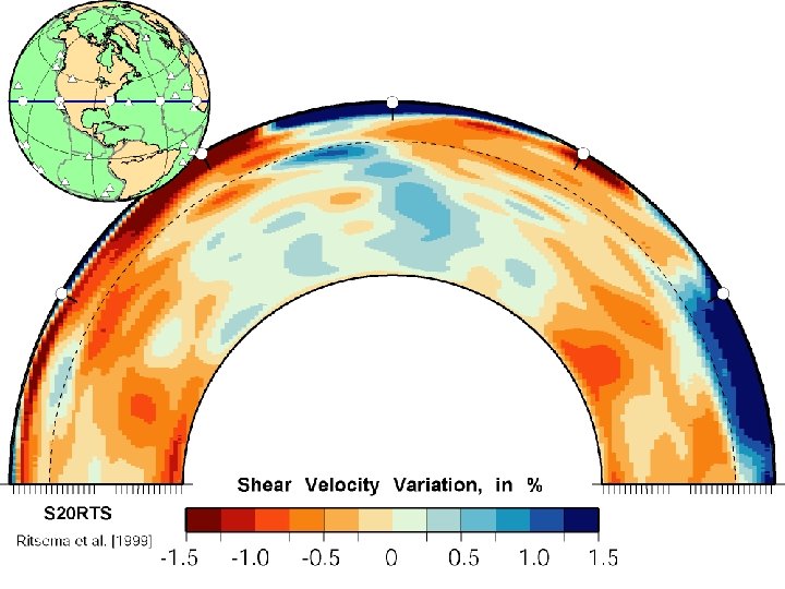
Example of a modern tomographic model S 40 RTS (Ritsema et al 2011)

Comparison of 3 -D shear velocity models Ritsema et al [2011] Simmons et al [2009] Kustowski et al [2008] Houser et al. [2008] Panning and Romanowicz [2006]

How fast are tomographic models improving?