RADAR Radial Applications Depiction Around Relations For DataCentric

RADAR: Radial Applications’ Depiction Around Relations For Data-Centric Ecosystems Panos Vassiliadis Univ. of Ioannina

Roadmap • • • Motivation & Related Work Problem Definition & Reference example Barycenter Methods Radial Methods Conclusions & Thoughts for the future 2

Data centric ecosystems & the need for a map Act 3 Act 4 Act 2 Act 5 WWW Act 1 3

Main drive We would like the administrators of the database, as well as the developers of all the software modules of the ecosystem to be able to have a visual overview of the ecosystem and to be able to understand the interdependencies between its parts. In simple words, the question can be expressed as: “how do we visualize a data -centric ecosystem? ”

Requirements and Challenges • Clear separation of relations and queries • Spatial memory – placing graph’s nodes that have semantic relationships closely over the diagram • Simple representation

PROBLEM DEFINITION 6

Graph model • The ecosystem is a bipartite graph G(V, E) – Nodes: relations and queries – Edges: query q uses a relation r in any way • Simplest possible model: we only care for the usage of a relation by a query • For the future – Query semantics – Views & constraints

Problem Definition • We need to lay the bipartite graph of the ecosystem on a 2 D surface (the screen) such that – Similar nodes are placed nearby (spatial memory) • We need to measure similarity – Dependency of queries over relations is easily traceable • Place queries as close to their defining relations – Clearly separate queries and relations 8

“Similar”? => Distance/Similarity function • Must precompute all possible distances between – two queries – two relations • We adopt a simple modeling and use Jaccard as the distance function

TPC-H as the reference example Q 1 Q 2 Q 3 Q 4 Q 5 Q 6 Q 7 Q 8 Q 9 Q 10 Q 11 Q 12 Q 13 Q 14 Q 15 Q 16 Q 17 Q 18 Q 19 Q 20 Q 21 Q 22 Region 0 1 0 0 0 0 Nation 0 1 0 1 1 1 0 0 0 0 1 1 0 Supplier Customer 0 0 1 1 1 1 1 0 0 0 0 1 0 1 0 0 1 Part 0 1 0 0 0 1 1 0 0 1 0 1 0 0 0 Partsupp Lineitem 0 1 1 0 0 1 0 1 0 1 1 1 0 0 0 1 1 0 0 1 0 1 1 1 0 0 Orders 0 0 1 1 1 1 0 0 1 0 0 1 1 10

11

BARYCENTER METHODS 12

Reference method for deploying bipartite graphs 1. Decide layers 2. Decide position of each node in its layer – Such that the number of edge crossings is minimized 3. Assign coordinates in the 2 D canvas 13

Reference method for deploying bipartite graphs 1. Decide layers 2. Decide position of each node in its layer – Such that the number of edge crossings is minimized 3. Assign coordinates in the 2 D canvas • In our case, steps 1 and 3 are easy; however step 2 is already NP-complete… 14

Barycenter methods • Recursive iterate the following over each layer of the bipartite graph – Given two layers L and L’, where L’ has an ordering for its nodes – Place each node of L as close as possible to the “middle” of the range of the nodes it accesses in layer L’, – “middle” can be • the median • the average (barycenter) of their positions 15

In our case • 2 layers: queries and relations • First align the relations by order of similarity • Then align the queries with respect to the placement of tables • We present only the sandwich extension: split the line of queries in two, surrounding the line of relations; place queries alternatively to the two lines 16

Align Tables as L 1 • Goal: place similar tables as close as possible – “similar”: hit by as many as possible common queries – Why? To reduce the span of these common queries 17

Align Tables as L 1 • While there exist relations not assigned to a position in the output list, the algorithm tries to find the two most similar relations out of the remaining ones, ri and rj, and once it finds them, it marks ri as max. I and rj as max. J. • Then, it places relation max. I to the sorted list’s next free slot and adds right next to it all the relations whose similarity to max. I is larger than a user-defined threshold τ (which is given as input parameter to the algorithm). • Practically, the sorted list contains sub-lists of relations, each with decreasing maximum similarity among its members. 18

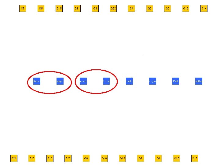
Align Tables as L 1 19

Nation-Supplier & Customer-Orders Q 1 Q 2 Q 3 Q 4 Q 5 Q 6 Q 7 Q 8 Q 9 Q 10 Q 11 Q 12 Q 13 Q 14 Q 15 Q 16 Q 17 Q 18 Q 19 Q 20 Q 21 Q 22 Region 0 1 0 0 0 0 Nation 0 1 0 1 1 1 0 0 0 0 1 1 0 Supplier Customer 0 0 1 1 1 1 1 0 0 0 0 1 0 1 0 0 1 Part 0 1 0 0 0 1 1 0 0 1 0 1 0 0 0 Partsupp Lineitem 0 1 1 0 0 1 0 1 0 1 1 1 0 0 0 1 1 0 0 1 0 1 1 1 0 0 Orders 0 0 1 1 1 1 0 0 1 0 0 1 1 20

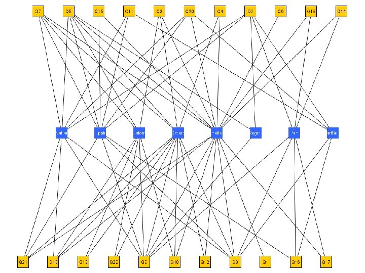
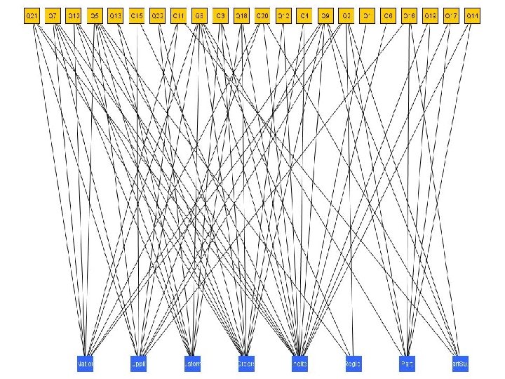
Coordinates • Once relations and queries are ordered, we give them coordinates • Y-coordinates fixed for both queries and relations • X-coordinates: – Relations: each relation is placed in the next slot (computed as a d. X step) in the x-axis – Queries have a barycenter computation: we add the x coordinates of all the relations accessed by the query and we divide this sum by the out-degree of the query. 22

RADIAL LAYOUTS 25

Basic idea • What if we bend the lines, to exploit the extra space? • Simple radial: – Inner circle for relations – Outer circle for queries Simple Radial 26

Concentric circles • What –if, instead of 1 query circle, we have many concentric circles? • Keeps clear separation of queries and relations • Scales better • Adapts to different semantics – – – One circle per query class … per source file / package / module … per developer … here: per query fan-out 27

Extra issues • Place each query as close to the relations if accesses • Handle gracefully the issue of large values for the range of accessed relations • Handle conflicts of nodes falling one on top of another 28

Algorithm Concentric Radial 29

Concentric Radial • We take as input – the graph of the ecosystem – the radius of the starting relations circle – the empty space among circles – a delta for conflicting queries • The output is a placement of queries and relations in a 2 D canvas 30

Concentric Radial • First, Align Tables as L 1, such that similar relations are placed one next to the other • Concert the relations’ line to circle, by computing the angle per relation • For each relation belonging to the next circle (here: depending on the fan-out), compute the arc of its accessing relations & place it in the bisector – If some relations are further than 180 o then, count the remainder angle • If there are conflicts, find the groups of conflicting nodes and push each of them by a small delta radius 31

Surprisingly, the most interesting part is the “movie” …MOVIE WITH SUBTITLES… 32

Fan-out = 1, 2 Things are nice and calm in radar city Observe the conflict resolution

Observe the angle Fan-out = 1, 2, 3

Fan-out = 1, 2, 3 See how the concentric circles work It’s called RADAR, remember?

Observe the angle Fan-out = 1, 2, 3, 4 Interestingly, things are still quite clear with 17/22 queries

Fan-out = 1, 2, 3, 4, 5 Then, heavy hitters come… A noisy guy

Fan-out = 1, 2, 3, 4, 5, 6 … and edges become more of a noise …

Done … and edges become more and more of a noise …

What have we gained? • Clear diagram – (to a large, but not full) extent • Less noise than barycenter • Scalability • … the movie … (!) – try it backwards • The visual clustering of queries (!) 40

Cluster: Q 14, Q 17, Q 19 41

CONCLUSIONS AND THOUGHTS FOR THE FUTURE 42

What we have done • Two methods for the visualization of data centric ecosystems, both with 2 variants – barycentric (here shown only the sandwich variant) – Radial – mainly interested to the concentric radial (or RADAR) • RADAR gives us better scalability, uses the empty space better, has multiple usages for its circles, clusters queries nicely and provides spatial memory 43

…but… • Heavy hitters make too much noise – Possibly stop adding edges after a threshold circle (remember: here fan-out determines the circle) – Unfortunately, agglomerative clustering of queries soon creates heavy hitters, too • Need for many real world examples to test scalability – Any input/suggestion/… is most welcome!! • Not yet incorporated in our impact analysis tool, HECATAEUS – http: //www. cs. uoi. gr/~pvassil/projects/hecataeus 44

…and… • More sophisticated modeling – of the graph (e. g. , with query semantics incorporated) – of the distance function – with views included – of both the logical (current) graph with its physical counterparts (i. e. , info on scripts, stored procedures, triggers, …) 45

Thank you! Questions? Many thanks go to our hosts and the W/S organizers

http: //www. cs. uoi. gr/~pvassil/projects /hecataeus 47