R v 1 c100 130 120 160 150
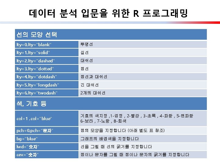

![데이터 분석 입문을 위한 R 프로그래밍 > v 1 [1] 100 130 120 160](https://slidetodoc.com/presentation_image_h/b1d4b36a147c6d1c6e5136cf8add0f8f/image-14.jpg "데이터 분석 입문을 위한 R 프로그래밍 > v 1 [1] 100 130 120 160")


 그래프에 범례 추가하기 legend(x 축 위치 ,")
 그룹으로 묶어서 가로로 출력시키기 - beside ,")
 여러 막대 그래프를 그룹으로 묶어서 한꺼번에 출력하기")
, main=\"Fruit's Sales QTY\" , +")
 하나의 막대 그래프에 여러 가지 내용을 한꺼번에")
 > qty BANANA CHERRY ORANGE")
 조건을 주고 그래프 그리기 peach 값이 200")
![데이터 분석 입문을 위한 R 프로그래밍 [ Bar plot 연습문제 1 답 ] >](https://slidetodoc.com/presentation_image_h/b1d4b36a147c6d1c6e5136cf8add0f8f/image-43.jpg "데이터 분석 입문을 위한 R 프로그래밍 [ Bar plot 연습문제 1 답 ] >")
![데이터 분석 입문을 위한 R 프로그래밍 [ Bar plot 연습문제 2 답 ] >](https://slidetodoc.com/presentation_image_h/b1d4b36a147c6d1c6e5136cf8add0f8f/image-45.jpg "데이터 분석 입문을 위한 R 프로그래밍 [ Bar plot 연습문제 2 답 ] >")
 히스토그램 그래프 그리기 : hist( ) >")
 히스토그램 그래프 그리기 : hist( ) >")
, oma=c(2, 2, 0. 1)) >")
 색깔과 label 명을 지정하기 > pie(p 1,")
 수치 값을 함께 출력하기 > pct <-")
 범례를 생략하고 그래프에 바로 출력하기 > pct")

, 2) y <- round(rnorm(30), 2)")
 관계도 그리기 : igraph( ) 함수 >")

 위 옵션에서 사용된 파라미터 값 정리 a)")
 점 관련 값 파라미터 의 미 vertex.")
 패키지 > >")


 > library(devtools) > install. packages(“d")

![데이터 분석 입문을 위한 R 프로그래밍 [ 범례 만들기 ] > lab <- names(total)](https://slidetodoc.com/presentation_image_h/b1d4b36a147c6d1c6e5136cf8add0f8f/image-91.jpg "데이터 분석 입문을 위한 R 프로그래밍 [ 범례 만들기 ] > lab <- names(total)")
 > value")

 3 D 챠트 그리기 > install. packages(\"plot")
 3 D 챠트 그리기 > attach(USArrests) >text")

 움직이는 3 D 챠트 그리기 – rgl")
![데이터 분석 입문을 위한 R 프로그래밍 [ 여러가지 rgl 패키지 예제들 ] example(surface 3](https://slidetodoc.com/presentation_image_h/b1d4b36a147c6d1c6e5136cf8add0f8f/image-105.jpg "데이터 분석 입문을 위한 R 프로그래밍 [ 여러가지 rgl 패키지 예제들 ] example(surface 3")
![데이터 분석 입문을 위한 R 프로그래밍 [ ggplot 2( ) 의 geom_함수들] > apropos("^geom*_")](https://slidetodoc.com/presentation_image_h/b1d4b36a147c6d1c6e5136cf8add0f8f/image-111.jpg "데이터 분석 입문을 위한 R 프로그래밍 [ ggplot 2( ) 의 geom_함수들] > apropos(\"^geom*_\")")
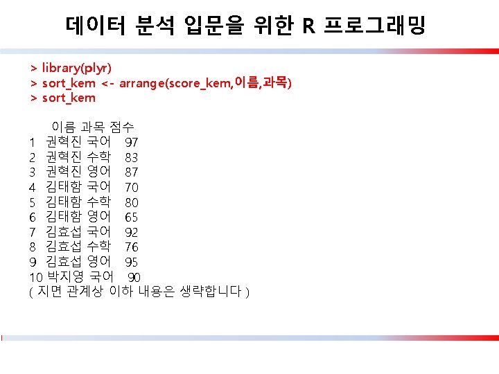
 패키지의 확장성 > ggplot(korean, aes(x=이름,")
![데이터 분석 입문을 위한 R 프로그래밍 > attributes(p) $names [1] "data" "layers" [6] "coordinates"](https://slidetodoc.com/presentation_image_h/b1d4b36a147c6d1c6e5136cf8add0f8f/image-115.jpg "데이터 분석 입문을 위한 R 프로그래밍 > attributes(p) $names [1] \"data\" \"layers\" [6] \"coordinates\"")
 geom_abline( ) : 그려진 그래프에 선을 추가하는")
 geom_bar( ) 함수 > b<-ggplot(korean, aes(x=이름, y=점수))")
) + geom_bar(stat=\"identity\", fill=\"green\", +")
) > c")
) > c")
) + geom_bar(stat=\"identity\",")
) + +")


) +")
 geom_boxplot( ) 함수 > > > +")
 geom_segment( ) 함수 > score <- read.")
))")
)) +")
 geom_point( ) 함수와 scatterplots > > install.")
)")
")
))")


,")
,")
")
")
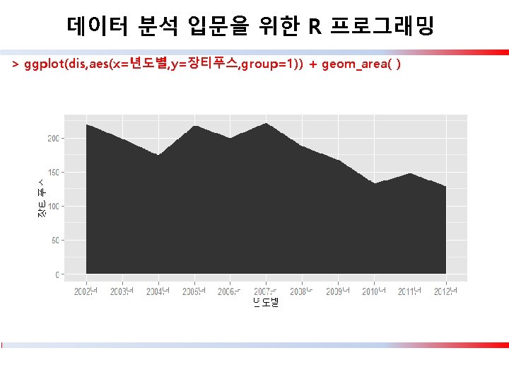
 geom_area( ) 함수 > dis <- read.")
) + + geom_area(color=\"red\",")
) + + geom_area(fill=\"cyan\",")
 geom_text( ) 함수 > korean <- read.")

- Slides: 159
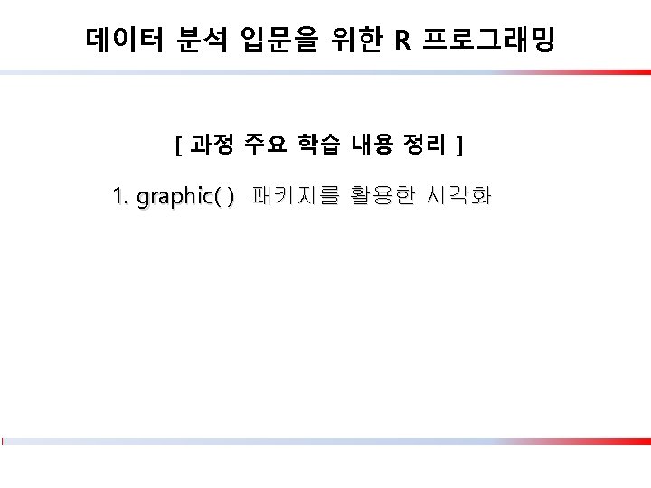
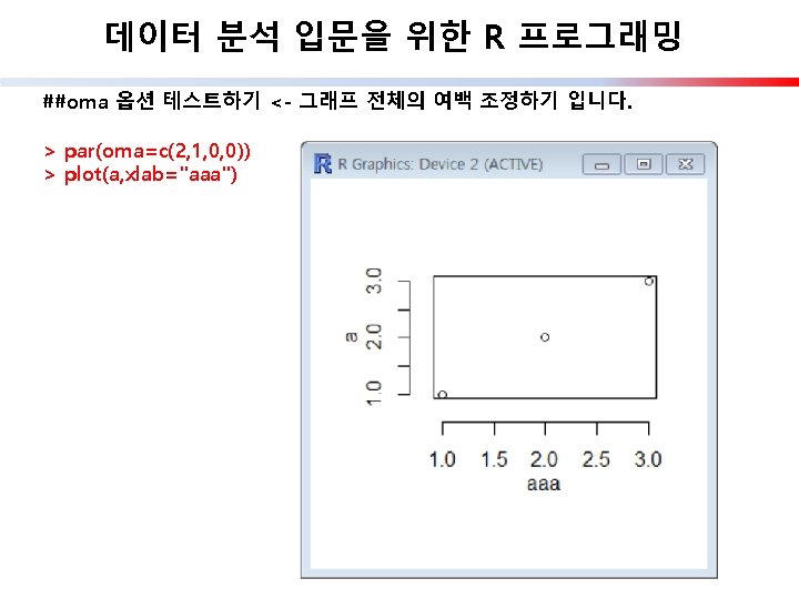
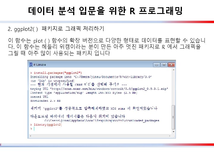
데이터 분석 입문을 위한 R 프로그래밍 > v 1 <- c(100, 130, 120, 160, 150) > plot(v 1, type='o', col='red', ylim=c(0, 200), axes=FALSE, ann=FALSE) > > axis(1, at=1: 5 , lab=c("MON", "TUE", "WED", "THU", "FRI")) > axis(2, ylim=c(0, 200)) > > title(main="FRUIT" , col. main="red", font. main=4) > title(xlab="DAY", col. lab="black") > title(ylab="PRICE", col. lab="blue")
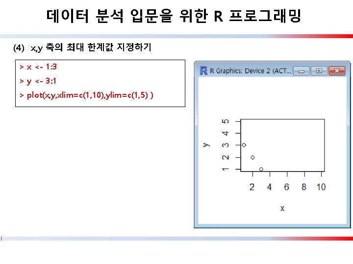
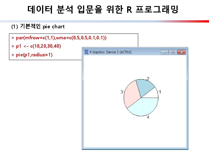
데이터 분석 입문을 위한 R 프로그래밍 > v 1 [1] 100 130 120 160 150 > par(mfrow=c(1, 3)) > pie(v 1) > plot(v 1, type="o") > barplot(v 1)
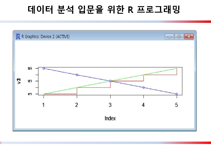
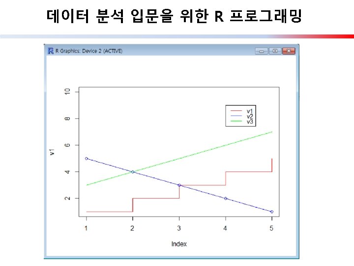
데이터 분석 입문을 위한 R 프로그래밍 > v 1 <- c(1, 2, 3, 4, 5) > v 2 <- c(5, 4, 3, 2, 1) > v 3 <- c(3, 4, 5, 6, 7) > plot(v 1, type="s", col="red", ylim=c(1, 10)) > lines(v 2, type="o", col="blue", ylim=c(1, 5)) > lines(v 3, type="l", col="green", ylim=c(1, 15))
데이터 분석 입문을 위한 R 프로그래밍 (10) 그래프에 범례 추가하기 legend(x 축 위치 , y 축 위치, 내용 , cex=글자크기 , col =색상 , pch=크기 , lty=선모양 > v 1 <- c(1, 2, 3, 4, 5) > v 2 <- c(5, 4, 3, 2, 1) > v 3 <- c(3, 4, 5, 6, 7) > plot(v 1, type="s", col="red", ylim=c(1, 10)) > lines(v 2, type="o", col="blue", ylim=c(1, 5)) > lines(v 3, type="l", col="green", ylim=c(1, 15)) > > legend(4, 9, c("v 1", "v 2", "v 3"), cex=0. 9, col=c("red", "blue", "green"), lty=1)
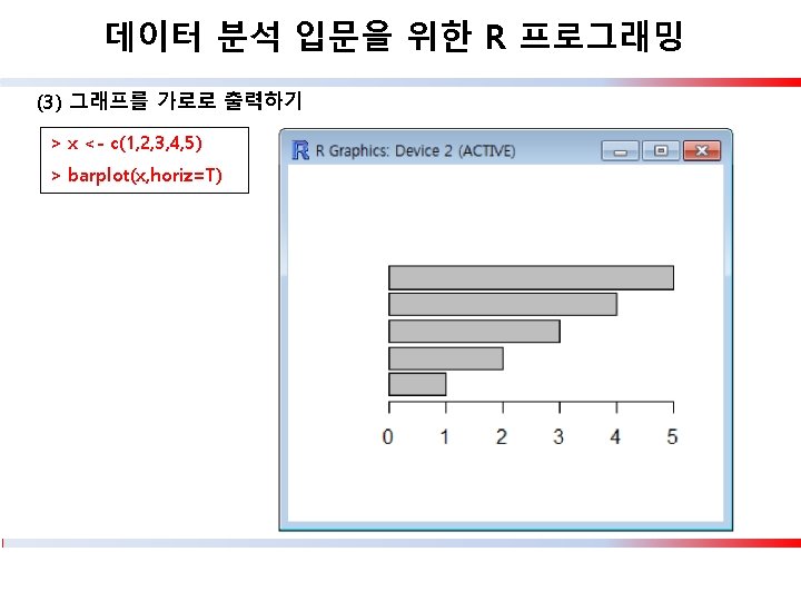
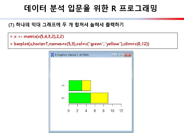
데이터 분석 입문을 위한 R 프로그래밍 (6) 그룹으로 묶어서 가로로 출력시키기 - beside , horiz=T 사용 > x <- matrix(c(5, 4, 3, 2), 2, 2) > par(oma=c(1, 0. 5, 1, 0. 5)) > barplot(x, names=c(5, 3), beside=T, col=c("green", "yellow"), horiz=T)
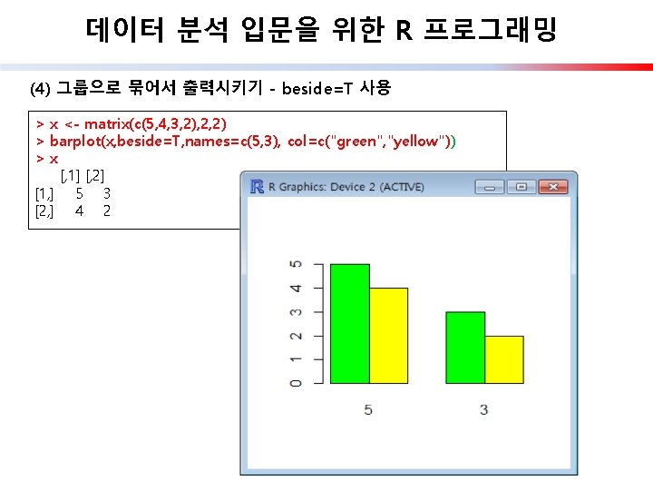
데이터 분석 입문을 위한 R 프로그래밍 (8) 여러 막대 그래프를 그룹으로 묶어서 한꺼번에 출력하기 > v 1 <- c(100, 120, 140, 160, 180) > v 2 <- c(120, 130, 150, 140, 170) > v 3 <- c(140, 170, 120, 110, 160) > qty <- data. frame(BANANA=v 1, CHERRY=v 2, ORANGE=v 3) > qty BANANA CHERRY ORANGE 1 100 120 140 2 120 130 170 3 140 150 120 4 160 140 110 5 180 170 160
데이터 분석 입문을 위한 R 프로그래밍 > barplot(as. matrix(qty), main="Fruit's Sales QTY" , + beside=T, col=rainbow(nrow(qty)), ylim=c(0, 400)) > legend(14, 400, c("MON", "TUE", "WED", "THU", "FRI"), cex=0. 8, fill=rainbow(nrow(qty)))
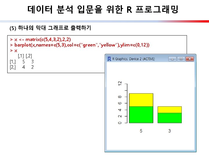
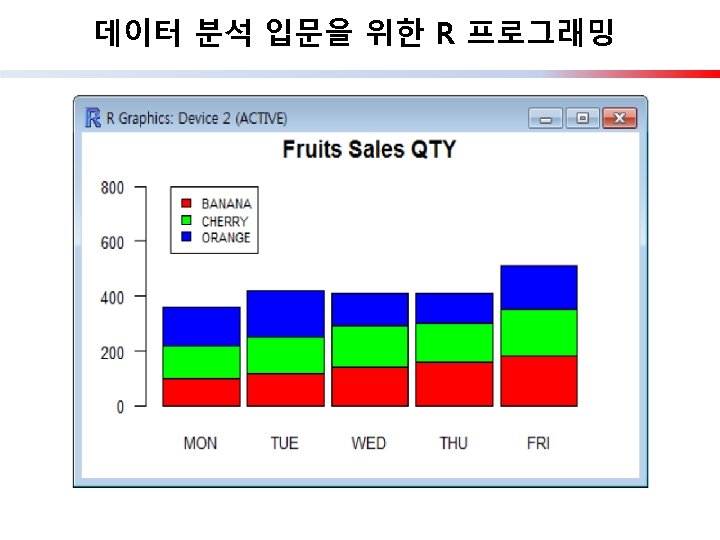
데이터 분석 입문을 위한 R 프로그래밍 (9) 하나의 막대 그래프에 여러 가지 내용을 한꺼번에 출력하기 > barplot(t(qty), main="Fruits Sales QTY", ylim=c(0, 900), + col=rainbow(length(qty)), space=0. 1, cex. axis=0. 8, las=1, + names. arg=c("MON", "TUE", "WED", "THU", "FRI"), cex=0. 8) > legend(0. 2, 800, names(qty), cex=0. 7, fill=rainbow(length(qty)) )
데이터 분석 입문을 위한 R 프로그래밍 전치행렬- t( ) > qty BANANA CHERRY ORANGE 1 100 120 140 2 120 130 170 3 140 150 120 4 160 140 110 5 180 170 160 > > t(qty) [, 1] [, 2] [, 3] [, 4] [, 5] BANANA 100 120 140 160 180 CHERRY 120 130 150 140 170 ORANGE 140 170 120 110 160
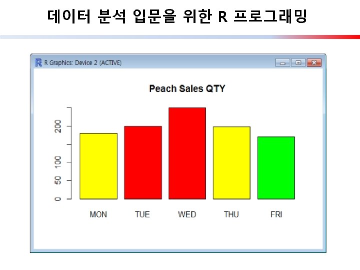
데이터 분석 입문을 위한 R 프로그래밍 (9) 조건을 주고 그래프 그리기 peach 값이 200 이상일 경우는 "red" , 180 - 199 는 "yellow" , 그 이하는 "green" 색으로 출력하세요. > peach <- c(180, 200, 250, 198, 170) > colors <- c( ) > for ( i in 1: length(peach)) + + + { if (peach[i] >= 200 ) { colors <- c(colors, "red") } else if ( peach[i] >= 180 ) { colors <- c(colors, "yellow") } else { colors <- c(colors, "green") } +} > barplot(peach, main="Peach Sales QTY" , + names. arg=c("MON", "TUE", "WED", "THU", "FRI"), col=colors)
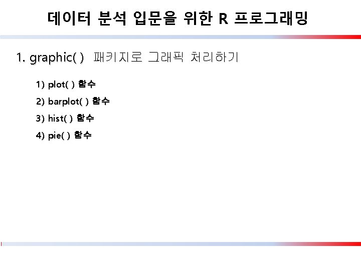
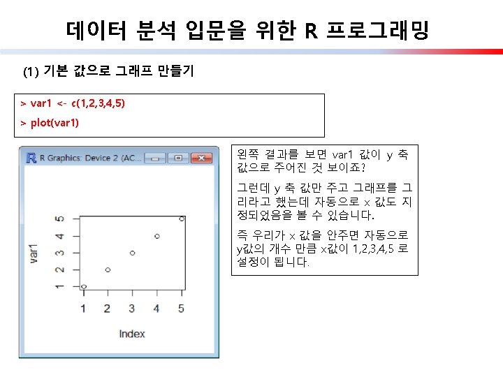
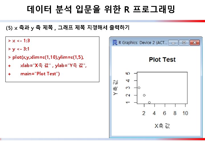
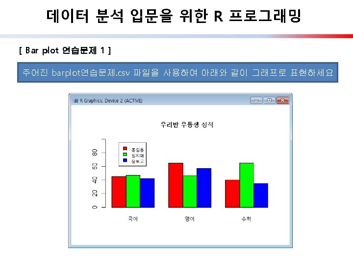
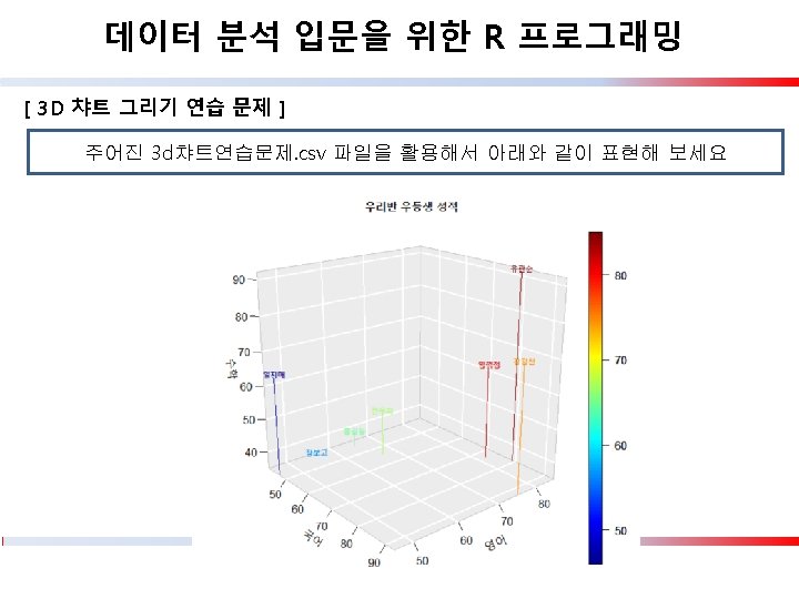
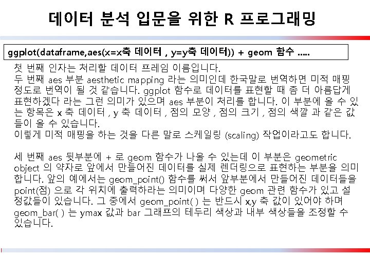
데이터 분석 입문을 위한 R 프로그래밍 [ Bar plot 연습문제 1 답 ] > var 1 <- read. csv("barplot연습문제. csv") > var 1 이름 국어 영어 수학 1 홍길동 45 65 40 2 일지매 47 46 65 3 장보고 42 57 35 > > par(oma=c(0, 0. 5, 0)) > > barplot(as. matrix(var 1[, c(2: 4)]), main="우리반 우등생 성적 + beside=T, col=rainbow(nrow(var 1)), ylim=c(0, 100)) > name <- var 1[, 1] > legend(1. 5, 95, name, cex=0. 8, fill=rainbow(nrow(var 1))) ",
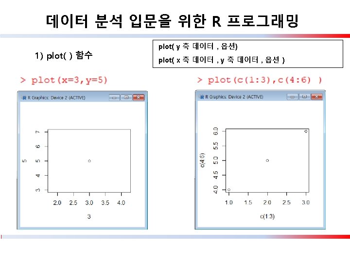
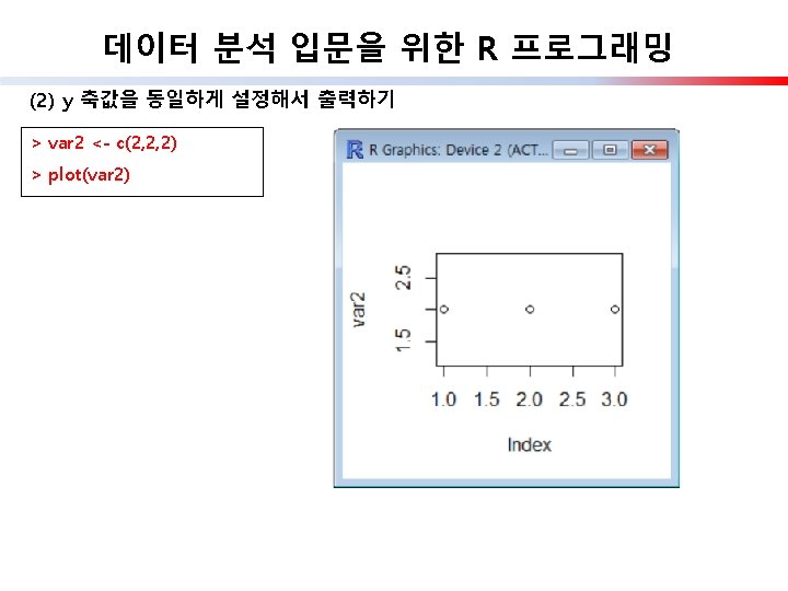
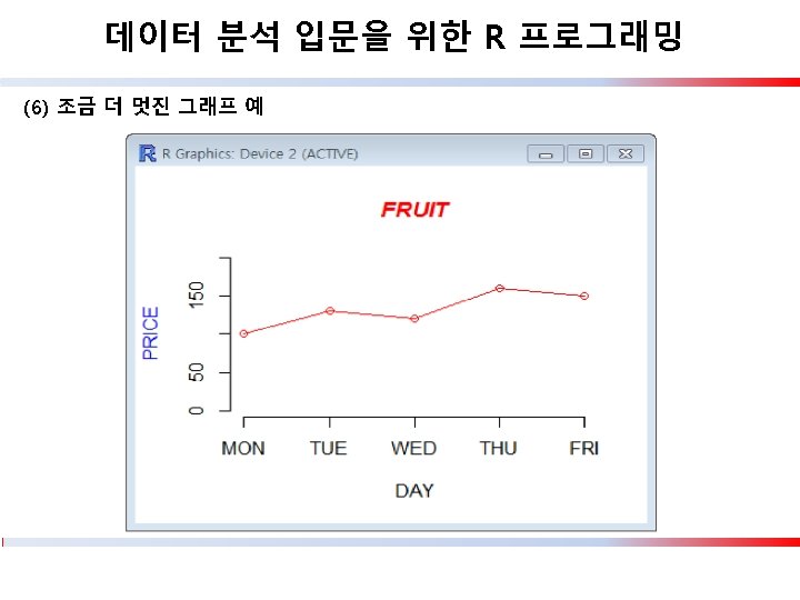
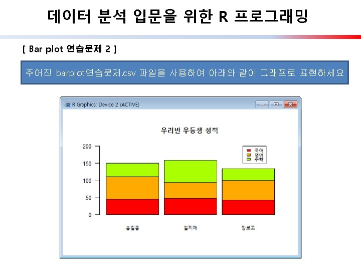
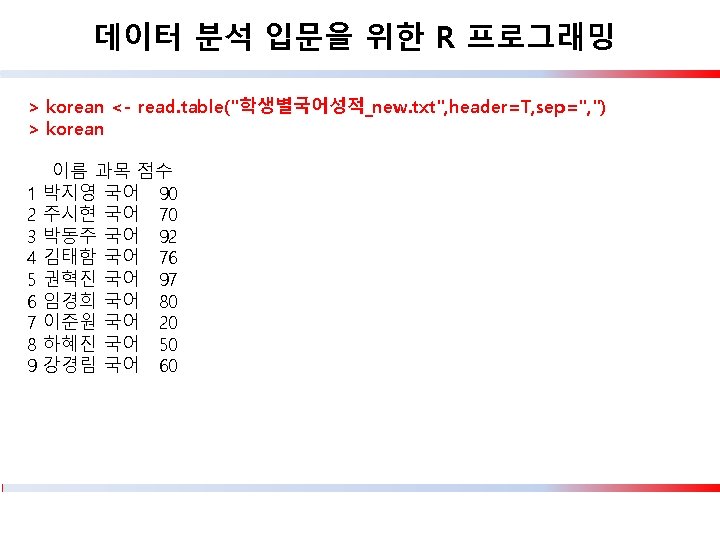
데이터 분석 입문을 위한 R 프로그래밍 [ Bar plot 연습문제 2 답 ] > var 2 <- as. matrix(var 1[, c(2: 4)]) > > barplot(t(var 2), main="우리반 우등생 성적 ", ylim=c(0, 200), + col=rainbow(length(var 2)), space=0. 1, cex. axis=0. 8, las=1, + names. arg=c("홍길동", "일지매", "장보고"), cex=0. 8) > > legend(2. 7, 200, (c("국어", "영어", "수학")), cex=0. 7, + fill=rainbow(length(var 2)))
데이터 분석 입문을 위한 R 프로그래밍 3) 히스토그램 그래프 그리기 : hist( ) > height <- c(182, 175, 167, 172, 163, 178, 181, 166, 159, 155) > hist(height, main="histogram of height")
데이터 분석 입문을 위한 R 프로그래밍 3) 히스토그램 그래프 그리기 : hist( ) > height <- c(182, 175, 167, 172, 163, 178, 181, 166, 159, 155) > pretty(height, 4) ## pretty 함수는 구간을 나누어 주는 함수 [1] 155 160 165 170 175 180 185 > hist(pretty(height, 4))
데이터 분석 입문을 위한 R 프로그래밍 > par(mfrow=c(1, 2), oma=c(2, 2, 0. 1)) > hist <- c(1, 1, 2, 3, 3, 3) > hist(hist) > plot(hist, main="Plot")
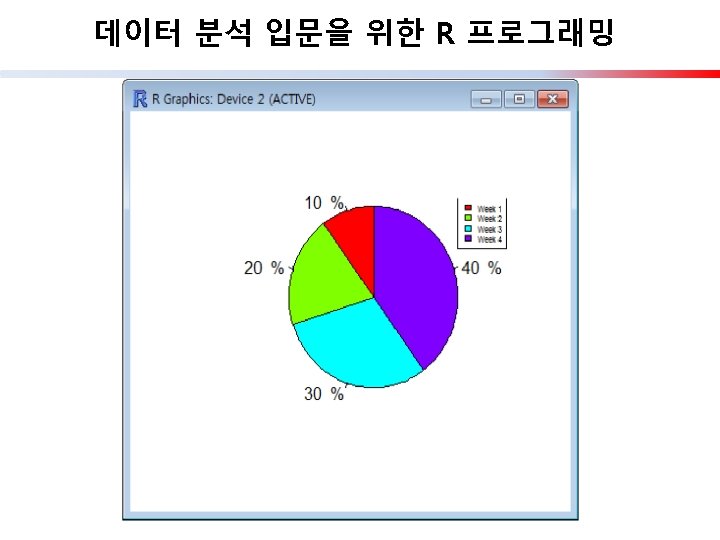
데이터 분석 입문을 위한 R 프로그래밍 (3) 색깔과 label 명을 지정하기 > pie(p 1, radius=1, init. angle=90, col=rainbow(length(p 1)), + label=c("Week 1" , "Week 2" , "Week 3" , "Week 4"))
데이터 분석 입문을 위한 R 프로그래밍 (4) 수치 값을 함께 출력하기 > pct <- round(p 1/sum(p 1) * 100, 1) > lab <- paste(pct, " %") > pie(p 1, radius=1, init. angle=90, col=rainbow(length(p 1)), + label=lab) > legend(1, 1. 1, c("Week 1", "Week 2", "Week 3", "Week 4"), + cex=0. 5, fill=rainbow(length(p 1)))
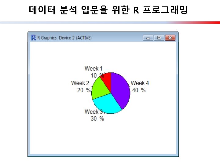
데이터 분석 입문을 위한 R 프로그래밍 (5) 범례를 생략하고 그래프에 바로 출력하기 > pct <- round(p 1/sum(p 1) * 100, 1) > lab 1 <- c("Week 1", "Week 2", "Week 3", "Week 4") > lab 2 <- paste(lab 1, "n", pct, " %") > pie(p 1, radius=1, init. angle=90, col=rainbow(length(p 1)), label=lab 2)
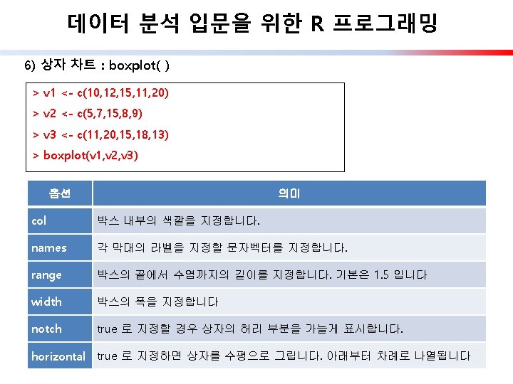
데이터 분석 입문을 위한 R 프로그래밍 > v 1 <- c(10, 12, 15, 11, 20) > v 2 <- c(5, 7, 15, 8, 9) > v 3 <- c(11, 20, 15, 18, 13) > boxplot(v 1, v 2, v 3, col=c("blue", "yellow", "pink"), + names=c("Blue", "Yellow", "Pink"), + horizontal=T)
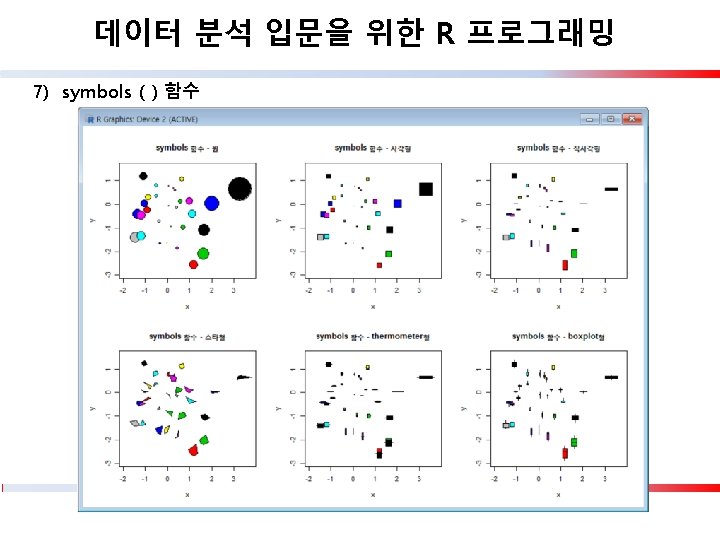
데이터 분석 입문을 위한 R 프로그래밍 x <- round(rnorm(30), 2) y <- round(rnorm(30), 2) var 1 var 2 var 3 var 4 var 5 <<<<<- abs(round(rnorm(30), 2)) round(runif(30), 2) par(mfrow=c(2, 3)) symbols(x, y, circles=abs(x), inches=0. 2, bg=1: 30) title(main="symbols 함수 - 원") symbols(x, y, squares=abs(x), inches=0. 2, bg=1: 30) title(main="symbols 함수 - 정사각형") symbols(x, y, rectangles=cbind(abs(x), abs(y)), inches=0. 2, bg=1: 30) title(main="symbols 함수 - 직사각형") symbols(x, y, stars=cbind(abs(x), abs(y), var 1, var 2, var 3), inches=0. 2, bg=1: 30) title(main="symbols 함수 - 스타형") symbols(x, y, thermometers=cbind(abs(x), abs(y), var 4), inches=0. 2, bg=1: 30) title(main="symbols 함수 - thermometer형") symbols(x, y, boxplots=cbind(abs(x), abs(y), var 3, var 4, var 5), inches=0. 2, bg=1: 30) title(main="symbols 함수 - boxplot형")
데이터 분석 입문을 위한 R 프로그래밍 8) 관계도 그리기 : igraph( ) 함수 > setwd("c: \a_temp") > install. packages("igraph") > library(igraph) > g 1 <- graph(c(1, 2, 2, 3, 2, 4, 1, 4, 5, 5, 3, 6)) > plot(g 1)
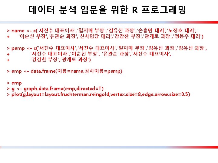
데이터 분석 입문을 위한 R 프로그래밍 화살표와 이름이 안 나오도록 설정하기 > g 3 <- graph. data. frame(emp, directed=F) > plot(g 3, layout=layout. fruchterman. reingold, vertex. size=8, + edge. arrow. size=0. 5 , vertex. label=NA)
데이터 분석 입문을 위한 R 프로그래밍 (1) 위 옵션에서 사용된 파라미터 값 정리 a) layout 관련 값 : layout. random , layout. cicle , layout. fruchterman. reingold , layout. kamada. kawai, layout. sprint , layout. lgl , layout. mds , layout. svd b) 선 관련 값 파라미터 의 미 edge. color 선의 색상 edge. lty 선 유형. solid , dashed , dotted edge. width 선의 폭 edge. label. family 선 종류. serif , sans , mono edge. arrow. size 화살의 크기 edge. arrow. width edge. label. font 화살의 폭 선 레이블 형, 1: 일반, 2: 볼드, 3: 이탤릭 4. 볼드 이텔릭 edge. arrow. mode 화살 머리 유형 edge. label. color 선 레이블 색상
데이터 분석 입문을 위한 R 프로그래밍 c) 점 관련 값 파라미터 의 미 vertex. size 점 크기 지정 vertex. color 점의 색 지정 vertex. frame. color 점 윤곽의 색 vertex. shape 점의 형태 vertex. label 점 레이블 vertex. label. family 점 레이블 종류 vertex. label. font 폰트 vertex. label. cex 점 레이블 크기 vertex. lebel. dist 점 중심과의 거리 vertex. label. degree 점 레이블 방향 vertex. label. color 점 레이블 색상
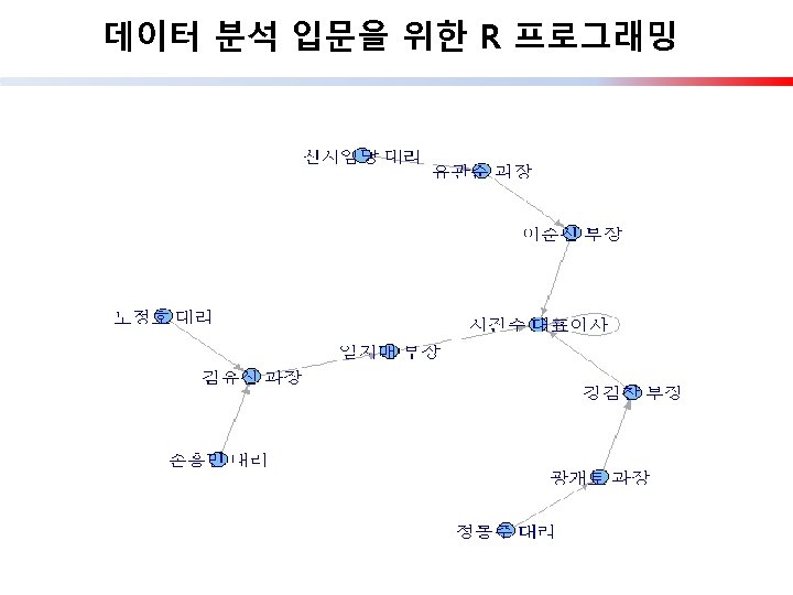
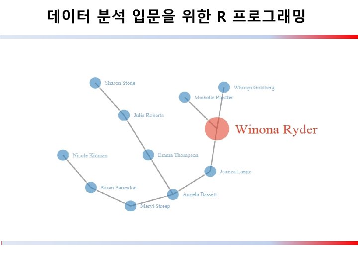
데이터 분석 입문을 위한 R 프로그래밍 - d 3 Network( ) 패키지 > > > + + + > > install. packages("devtools") library(devtools) install_github("christophergandrud/d 3 Network") library(RCurl) library(d 3 Network) name <- c('Angela Bassett', 'Jessica Lange', 'Winona Ryder', 'Michelle Pfeiffer', 'Whoopi Goldberg', 'Emma Thompson', 'Julia Roberts', 'Sharon Stone', 'Meryl Streep', 'Susan Sarandon', 'Nicole Kidman') pemp <- c('Angela Bassett', 'Jessica Lange', 'Winona Ryder', 'Angela Bassett', 'Emma Thompson', 'Julia Roberts', 'Angela Bassett', 'Meryl Streep', 'Susan Sarandon') emp <- data. frame(이름=name, 상사이름=pemp) d 3 Simple. Network(emp, width=600, height=600, file="c: \ a_temp\d 3. html")
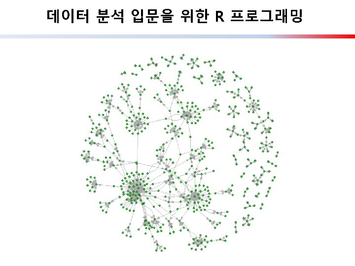
데이터 분석 입문을 위한 R 프로그래밍 - 군집분석 표현하기 > g <- read. csv("군집분석. csv", head=T) > graph <- data. frame(학생=g$학생, 교수=g$교수) > g<-graph. data. frame(graph, directed=T) > plot(g, layout=layout. fruchterman. reingold, vertex. size=2, edge. arrow. size=0. 5, + vertex. color="green", vertex. label=NA)
데이터 분석 입문을 위한 R 프로그래밍 > plot(g, layout=layout. kamada. kawai, vertex. size=2, edge. arrow. size=0. 5, + vertex. label=NA)
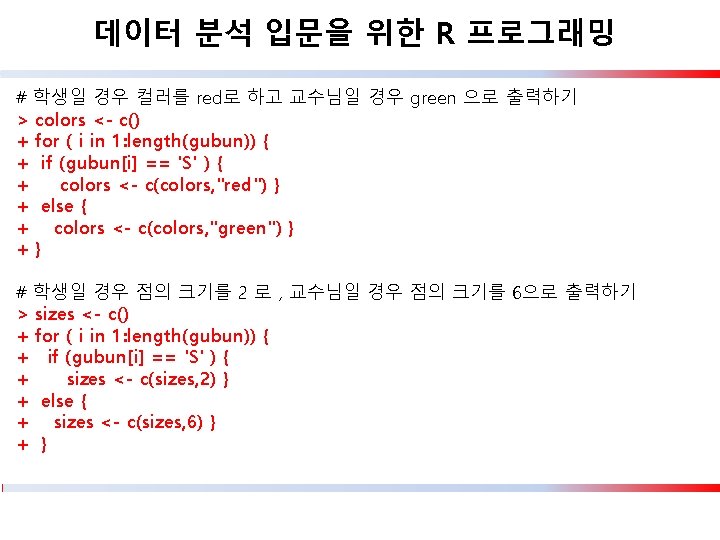
데이터 분석 입문을 위한 R 프로그래밍 # 학생과 교수의 색상과 크기를 구분해서 출력하기 > g<-read. csv("군집분석. csv", head=T) > graph <- data. frame(학생=g$학생, 교수=g$교수) > g <- graph. data. frame(graph, directed=T) >g > V(g)$name > gubun 1 <- V(g)$name > gubun 1 > gubun <- str_sub(gubun 1, start=1, end=1) > gubun
데이터 분석 입문을 위한 R 프로그래밍 > plot(g, layout=layout. fruchterman. reingold, vertex. size=sizes, edge. arrow. size=0. 5, + vertex. color=colors)
데이터 분석 입문을 위한 R 프로그래밍 # 이름 없애기 – 위 그래프에서 이름부분이 너무 지저분해서 이름을 제거하고 출력하기 > plot(g, layout=layout. fruchterman. reingold, vertex. size=sizes, edge. arrow. size=0. 5, + vertex. color=colors, vertex. label=NA)
데이터 분석 입문을 위한 R 프로그래밍 # 화살표 표시 없게 만들기 > plot(g, layout=layout. fruchterman. reingold, vertex. size=sizes, edge. arrow. size=0, + vertex. color=colors, vertex. label=NA)
데이터 분석 입문을 위한 R 프로그래밍 # 학생과 교수의 도형 모양 다르게 하고 화살표 없애고 색깔도 다르게 하기 > plot(g, layout=layout. kamada. kawai, vertex. size=sizes, edge. arrow. size=0, + , vertex. color=colors, vertex. label=NA)
데이터 분석 입문을 위한 R 프로그래밍 # 아래 코드는 교수님일 경우 모양을 square 로 하고 # 교수님일 경우 점의 모양을 circle 로 하는 코드임 > shapes <- c() > for ( i in 1: length(gubun)) { + if (gubun[i] == 'S' ) { + shapes <- c(shapes, "circle") } + else { + shapes <- c(shapes, "square") } +} > plot(g, layout=layout. kamada. kawai, vertex. size=sizes, edge. arrow. size=0, + , vertex. color=colors, vertex. label=NA, vertex. shape=shapes)
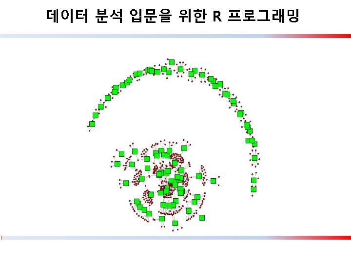
데이터 분석 입문을 위한 R 프로그래밍 > install. packages("devtools") > library(devtools) > install. packages(“d 3 Network”) > library(d 3 Network) > virus 1 <- read. csv("메르스전염현황. csv", header=T) > d 3 Simple. Network(virus 1, width=600, height=600, + file="c: \r_temp\mers. html")
데이터 분석 입문을 위한 R 프로그래밍 [ 범례 만들기 ] > lab <- names(total) > value <- table(lab) Ø value > pie(value, labels=lab, radius=0. 1, cex=0. 6, col=NA)
데이터 분석 입문을 위한 R 프로그래밍 범례 만들기 > label <- names(total) > value <- table(label) > color <- c("black", "red", "green", "blue", "cyan", "violet") > pie(value, labels=label, col=color, radius=0. 1, cex=0. 6)
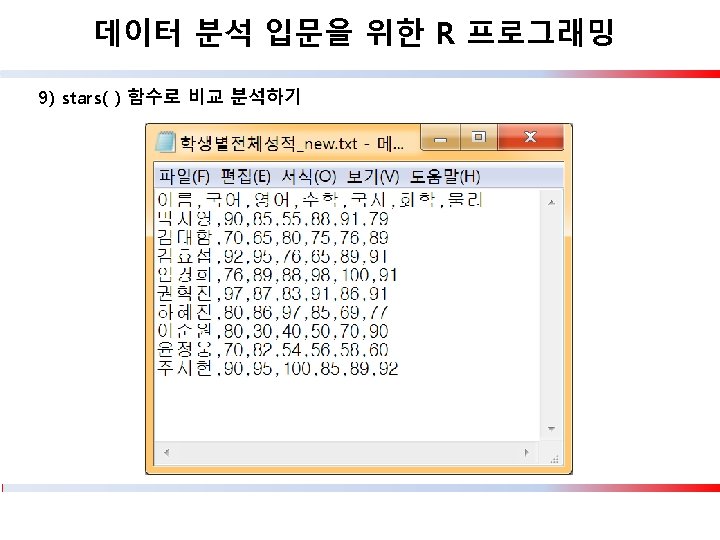
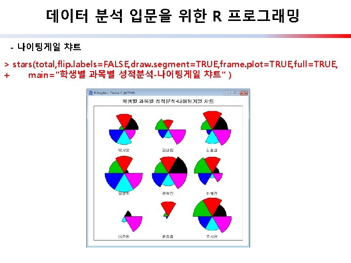
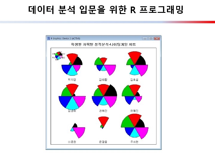
데이터 분석 입문을 위한 R 프로그래밍 > stars(total, flip. labels=FALSE, draw. segment=TRUE, frame. plot=TRUE, full=FALSE, + main="학생별 과목별 분석 다이어그램-반원챠트" )
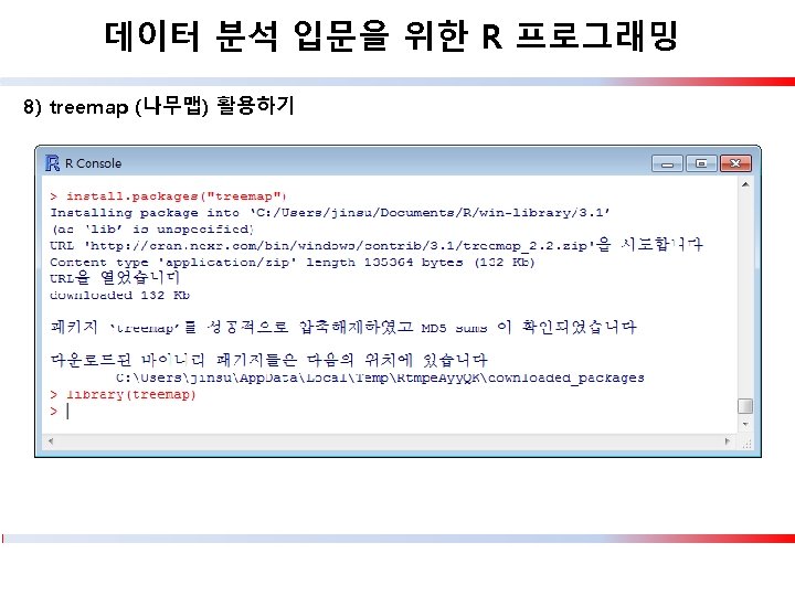
데이터 분석 입문을 위한 R 프로그래밍 11) 3 D 챠트 그리기 > install. packages("plot 3 D") > library(plot 3 D) > par(mar=c(1, 1, 1, 1)) > scatter 3 D(mtcars$wt, y=mtcars$gear, + z=mtcars$mpg, pch=19)
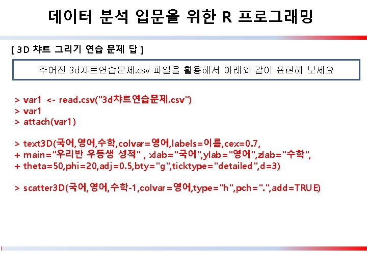
데이터 분석 입문을 위한 R 프로그래밍 11) 3 D 챠트 그리기 > attach(USArrests) >text 3 D(Murder, Assault, Rape, colvar=Urban. Pop, labels=rownames(USArrests), + cex=0. 7, main="USA arrests" , xlab="Murder", ylab="Assault", zlab="Rape", + theta=30, phi=20, clab=c("Urban", "Pop"), adj=0. 5, bty="g“ , + ticktype="detailed", d=3) > scatter 3 D(Murder, Assault, Rape, colvar=Urban. Pop, type="h", + pch=". ", add=TRUE)
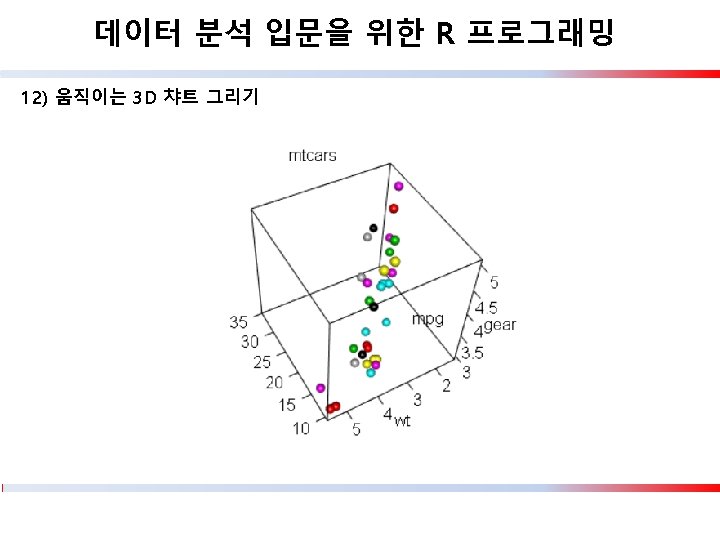
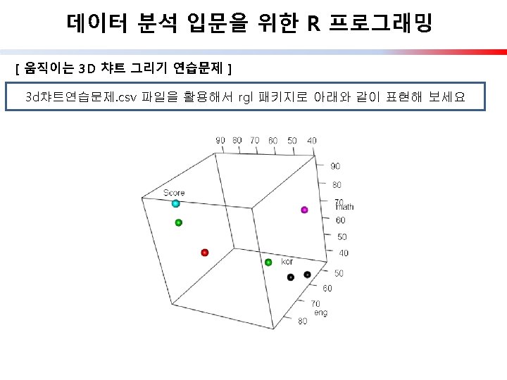
데이터 분석 입문을 위한 R 프로그래밍 11) 움직이는 3 D 챠트 그리기 – rgl 패키지 활용하기 > install. packages("rgl") > library(rgl) > attach(mtcars) > plot 3 d(x=wt, y=gear, z=mpg, col=mpg, size=2, type="s", + main="mtcars", xlab="wt", ylab="gear", zlab="mpg")
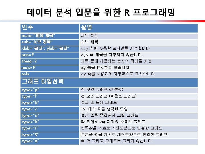
데이터 분석 입문을 위한 R 프로그래밍 [ 여러가지 rgl 패키지 예제들 ] example(surface 3 d) demo(abundance) http: //rgl. neoscientists. org/gallery. shtml
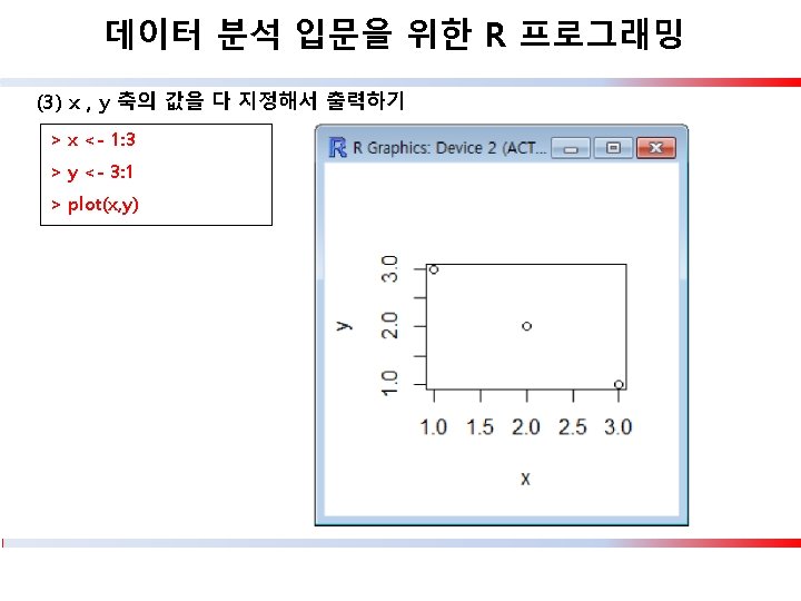
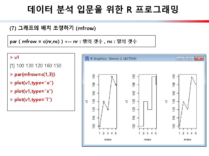
데이터 분석 입문을 위한 R 프로그래밍 [ ggplot 2( ) 의 geom_함수들] > apropos("^geom*_") [1] "geom_abline" "geom_area" "geom_bar" "geom_bin 2 d" [5] "geom_blank" "geom_boxplot" "geom_contour" "geom_count" [9] "geom_crossbar" "geom_curve" "geom_density_2 d" [13] "geom_density 2 d" "geom_dotplot" "geom_errorbarh" [17] "geom_freqpoly" "geom_hex" "geom_histogram" "geom_hline" [21] "geom_jitter" "geom_label" "geom_linerange" [25] "geom_map" "geom_path" "geom_pointrange" [29] "geom_polygon" "geom_qq" "geom_quantile" "geom_raster" [33] "geom_rect" "geom_ribbon" "geom_rug" "geom_segment" [37] "geom_smooth" "geom_spoke" "geom_step" "geom_text" [41] "geom_tile" "geom_violin" "geom_vline"
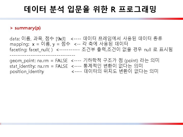
데이터 분석 입문을 위한 R 프로그래밍 ggplot 2( ) 패키지의 확장성 > ggplot(korean, aes(x=이름, y=점수)) + geom_point( ) > ggplot(korean, aes(x=이름, y=점수, group=과목)) + geom_line( ) > ggplot(korean, aes(x=이름, y=점수)) + geom_bar(stat="identity")
데이터 분석 입문을 위한 R 프로그래밍 > attributes(p) $names [1] "data" "layers" [6] "coordinates" "facet" $class [1] "gg" "ggplot" "scales" "mapping" "plot_env" "labels" "theme"
데이터 분석 입문을 위한 R 프로그래밍 2) geom_abline( ) : 그려진 그래프에 선을 추가하는 함수 > l <- ggplot(korean, aes(x=이름, y=점수, group=과목)) + geom_line( ) > l + geom_abline(intercept=50, slope=0, color="green")
데이터 분석 입문을 위한 R 프로그래밍 3) geom_bar( ) 함수 > b<-ggplot(korean, aes(x=이름, y=점수)) + geom_bar(stat="identity") >b
데이터 분석 입문을 위한 R 프로그래밍 > ggplot(korean, aes(x=이름, y=점수)) + geom_bar(stat="identity", fill="green", + colour="red")
데이터 분석 입문을 위한 R 프로그래밍 > b <- ggplot(korean, aes(x=이름, y=점수)) > c <- b + geom_bar(stat="identity", fill="green", colour="red") > c + coord_flip( )
데이터 분석 입문을 위한 R 프로그래밍 > b <- ggplot(korean, aes(x=이름, y=점수)) > c <- b + geom_bar(stat="identity", fill="green", colour="red") > c + facet_wrap( ~ 이름 )
데이터 분석 입문을 위한 R 프로그래밍 > gg <- ggplot(korean, aes(x=이름, y=점수)) + geom_bar(stat="identity", fill="green", + colour="red") > gg + theme(axis. text. x=element_text(angle=45, hjust=1, vjust=1, + color="blue", size=8))
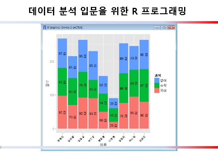
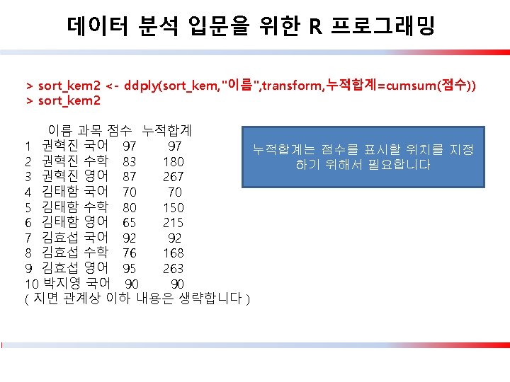
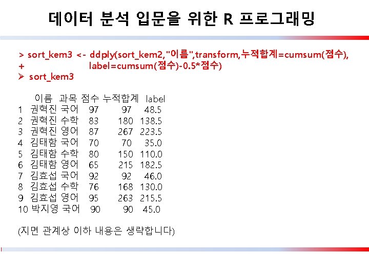
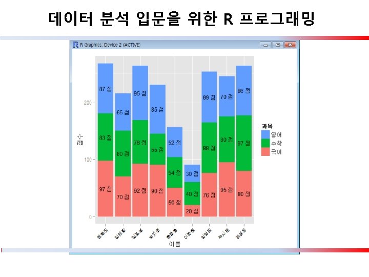
데이터 분석 입문을 위한 R 프로그래밍 > ggplot(sort_kem 3, aes(x=이름, y=점수, fill=과목)) + + geom_bar(stat="identity") + + geom_text(aes(y=label, label=paste(점수, '점')), colour="black", size=4) 그런데 순서가?
데이터 분석 입문을 위한 R 프로그래밍 > gg 2 <- ggplot(sort_kem 3, aes(x=이름, y=점수, fill=과목)) + + geom_bar(stat="identity") + + geom_text(aes(y=label, label=paste(점수, '점')), colour="black", size=4) + + guides(fill=guide_legend(reverse=T)) > > gg 2 + theme(axis. text. x=element_text(angle=45, hjust=1, vjust=1, + colour="black", size=8))
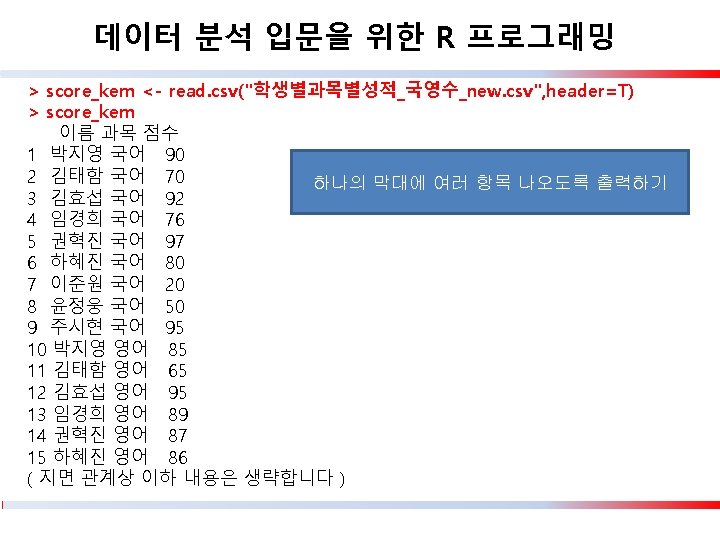
데이터 분석 입문을 위한 R 프로그래밍 > > > + > score_kem <- read. csv("학생별과목별성적_국영수_new. csv", header=T) b <- ggplot(score_kem, aes(x=이름, y=점수)) c <- b + geom_bar(stat="identity", fill="green", colour="red")+ theme(axis. text. x = element_blank()) c + facet_wrap( ~ 이름+과목 )
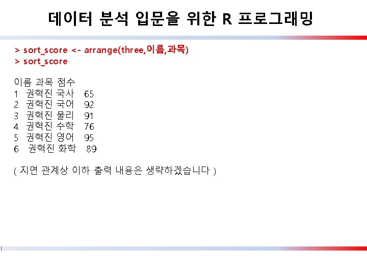
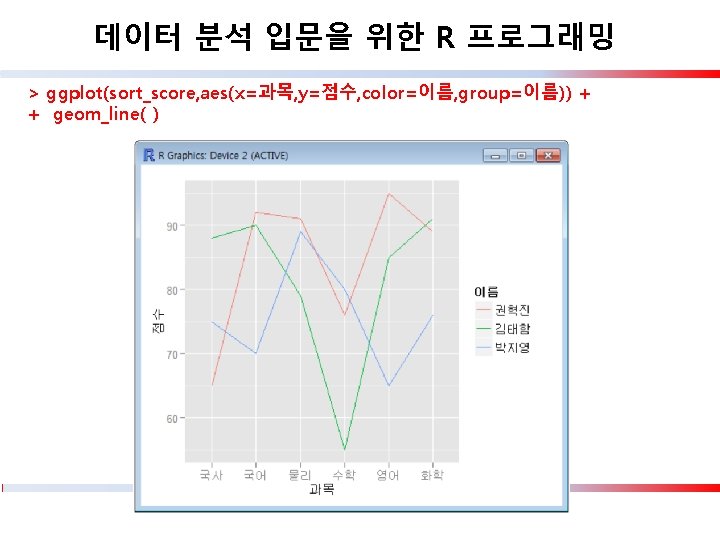
데이터 분석 입문을 위한 R 프로그래밍 > ggplot(sort_score, aes(x=과목, y=점수, color=이름, group=이름, fill=이름)) + + geom_line( ) + geom_point(size=6, shape=22 )
데이터 분석 입문을 위한 R 프로그래밍 5) geom_boxplot( ) 함수 > > > + s_temp <- read. csv("서울의기온변화. csv") s_temp ggplot(s_temp, aes(factor(Month), Mean. Temp)) + geom_boxplot(aes(fill=factor(Month)))
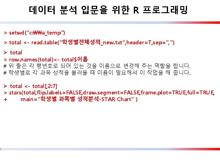
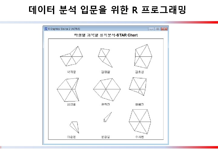
데이터 분석 입문을 위한 R 프로그래밍 6) geom_segment( ) 함수 > score <- read. table("학생별전체성적_new. txt", header=T, sep=", ") > score 1 2 3 4 5 6 7 8 9 이름 국어 영어 수학 국사 화학 물리 박지영 90 85 55 88 91 79 김태함 70 65 80 75 76 89 김효섭 92 95 76 65 89 91 임경희 76 89 88 98 100 91 권혁진 97 87 83 91 86 91 하혜진 80 86 97 85 69 77 이준원 80 30 40 50 70 90 윤정웅 70 82 54 56 58 60 주시현 90 95 100 85 89 92
데이터 분석 입문을 위한 R 프로그래밍 > + + + ggplot(score, aes(x=영어, y=reorder(이름, 영어))) + geom_point(size=6) + theme_bw( ) + theme(panel. grid. major. x=element_blank( ) , panel. grid. minor. x=element_blank( ) , panel. grid. major. y=element_line(color="red", linetype="dashed"))
데이터 분석 입문을 위한 R 프로그래밍 > + + ggplot(score, aes(x=영어, y=reorder(이름, 영어))) + geom_segment(aes(yend=이름), xend=0, color="blue") + geom_point(size=6, color="green") + theme_bw() + theme(panel. grid. major. y=element_blank())
데이터 분석 입문을 위한 R 프로그래밍 7) geom_point( ) 함수와 scatterplots > > install. packages("grid. Extra") library(grid. Extra) v_mt <- mtcars v_mt mpg cyl disp hp drat wt qsec vs am gear carb Mazda RX 4 21. 0 6 160. 0 110 3. 90 2. 620 16. 46 0 1 4 4 Mazda RX 4 Wag 21. 0 6 160. 0 110 3. 90 2. 875 17. 02 0 1 4 4 Datsun 710 22. 8 4 108. 0 93 3. 85 2. 320 18. 61 1 1 4 1 Hornet 4 Drive 21. 4 6 258. 0 110 3. 08 3. 215 19. 44 1 0 3 1 Hornet Sportabout 18. 7 8 360. 0 175 3. 15 3. 440 17. 02 0 0 3 2 Valiant 18. 1 6 225. 0 105 2. 76 3. 460 20. 22 1 0 3 1 Duster 360 14. 3 8 360. 0 245 3. 21 3. 570 15. 84 0 0 3 4 ( 지면 관계상 이하 내용은 생략하겠습니다.
데이터 분석 입문을 위한 R 프로그래밍 > graph 1 <- ggplot(v_mt, aes(x=hp , y=mpg)) > graph 1 + geom_point() > save. Plot("graph 1. png", type="png")
데이터 분석 입문을 위한 R 프로그래밍 > graph 2 <- graph 1 + geom_point(colour="blue") - 색상 변경하기 > graph 2 > save. Plot("graph 2. png", type="png")
데이터 분석 입문을 위한 R 프로그래밍 > graph 3 <- graph 2 + geom_point(aes(color=factor(am))) - 종류별로 다른 색상 지정 하기 > graph 3 > save. Plot("graph 3. png", type="png")
데이터 분석 입문을 위한 R 프로그래밍 > graph 4 <- graph 1 + geom_point(size = 7) - 크기 지정하기 > graph 4 > save. Plot("graph 4. png", type="png")
데이터 분석 입문을 위한 R 프로그래밍 > graph 5 <- graph 1 + geom_point(aes(size = wt)) - 값 별로 다른 크기 지정하기 > graph 5 > save. Plot("graph 5. png", type="png")
데이터 분석 입문을 위한 R 프로그래밍 > graph 6 <- graph 1 + geom_point(aes(shape=factor(am), size = wt)) > graph 6 > save. Plot("graph 6. png", type="png") - 종류별로 크기와 모양 지정하기
데이터 분석 입문을 위한 R 프로그래밍 > graph 7 <- graph 1 + geom_point(aes(shape=factor(am), color=factor(am), size = wt)) + + scale_color_manual(values=c("red", "green")) > graph 7 > save. Plot("graph 7. png", type="png") - 종류별로 크기, 모양, 색상 지정하기
데이터 분석 입문을 위한 R 프로그래밍 > graph 8 <- graph 1 + geom_point(color="red") + geom_line() - 선 추가하기 > graph 8 > save. Plot("graph 8. png", type="png")
데이터 분석 입문을 위한 R 프로그래밍 > graph 9 <- graph 1 + geom_point(color="blue") + + labs(x="마력" , y="연비(mile/gallon)") > graph 9 - x 축과 y 축 이름 바꾸기 > save. Plot("graph 9. png", type="png")
데이터 분석 입문을 위한 R 프로그래밍 8) geom_area( ) 함수 > dis <- read. csv("1군전염병발병현황_년도별. csv", strings. As. Factors=F) > dis 년도별 콜레라 장티푸스 이질 대장균 A형간염 1 2002년 4 221 767 8 0 2 2003년 1 199 1117 52 0 3 2004년 10 174 487 118 0 4 2005년 16 219 317 43 0 5 2006년 5 200 389 37 0 6 2007년 7 223 131 41 0 7 2008년 5 188 209 58 0 8 2009년 0 168 180 62 0 9 2010년 8 133 228 56 0 10 2011년 3 148 171 71 5521 11 2012년 0 129 90 58 1197
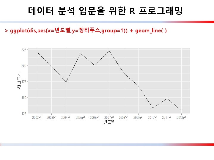
데이터 분석 입문을 위한 R 프로그래밍 > ggplot(dis, aes(x=년도별, y=장티푸스, group=1)) + + geom_area(color="red", fill="cyan", alpha=0. 4)
데이터 분석 입문을 위한 R 프로그래밍 > ggplot(dis, aes(x=년도별, y=장티푸스, group=1)) + + geom_area(fill="cyan", alpha=0. 4) + geom_line( )
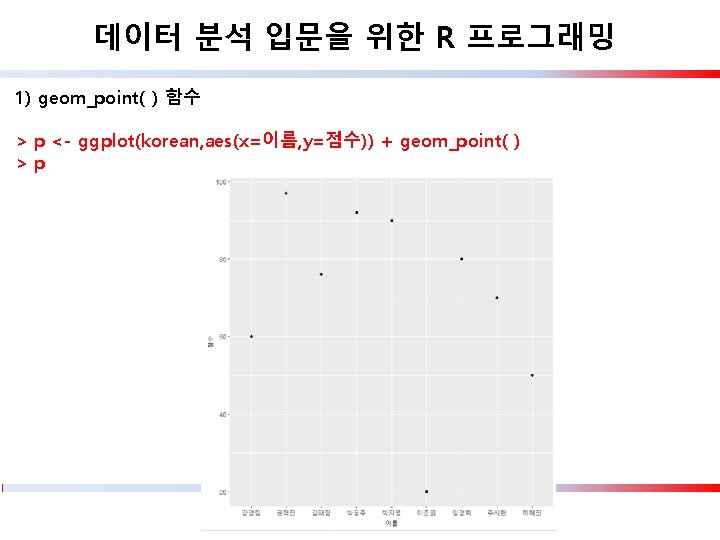
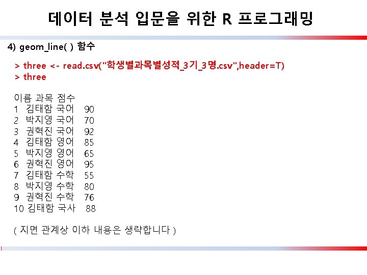
데이터 분석 입문을 위한 R 프로그래밍 9) geom_text( ) 함수 > korean <- read. table("학생별국어성적_new. txt", header=T, sep=", ") > p <- ggplot(korean, aes(x=이름, y=점수, label=이름)) + geom_point( ) > p + geom_text(color=rainbow(length(korean$이름)), size=3, hjust=1)