R Programming Language INTRODUCTION HISTORY DATA TYPES STATISTICS

R Programming Language INTRODUCTION – HISTORY, DATA TYPES, STATISTICS, USES

History Of R R is a programming language and software environment for statistical analysis, graphics representation and reporting. R was created by Ross Ihaka and Robert Gentleman at the University of Auckland, New Zealand, and is currently developed by the R Development Core Team. The core of R is an interpreted computer language which allows branching and looping as well as modular programming using functions. R allows integration with the procedures written in the C, C++, . Net, Python or FORTRAN languages for efficiency.

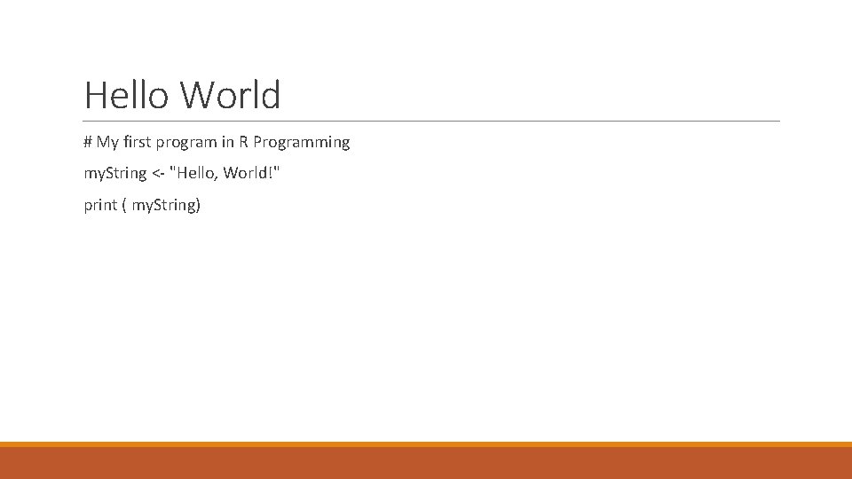
Hello World # My first program in R Programming my. String <- "Hello, World!" print ( my. String)

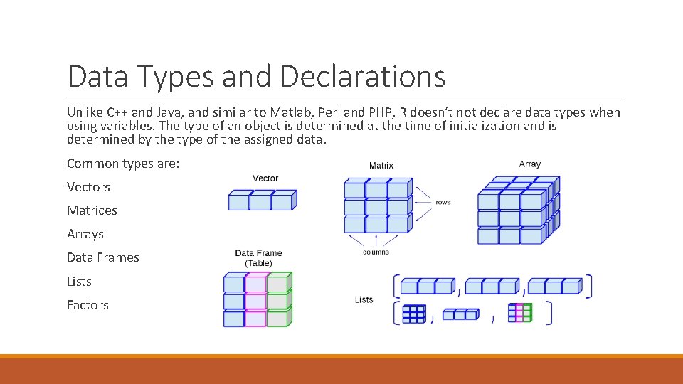
Data Types and Declarations Unlike C++ and Java, and similar to Matlab, Perl and PHP, R doesn’t not declare data types when using variables. The type of an object is determined at the time of initialization and is determined by the type of the assigned data. Common types are: Vectors Matrices Arrays Data Frames Lists Factors

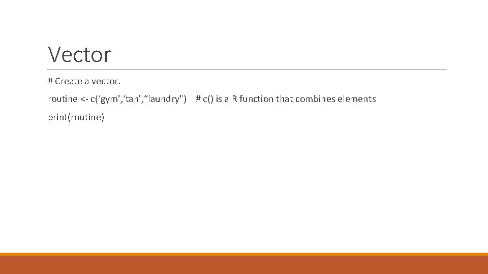
Vector # Create a vector. routine <- c(‘gym', ‘tan', “laundry") # c() is a R function that combines elements print(routine)

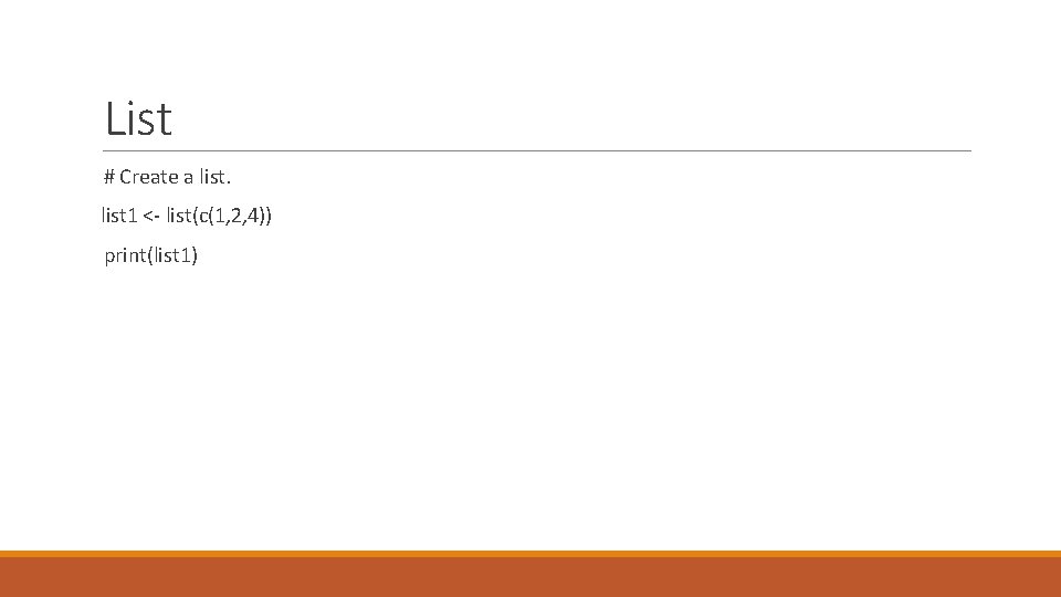
List # Create a list 1 <- list(c(1, 2, 4)) print(list 1)

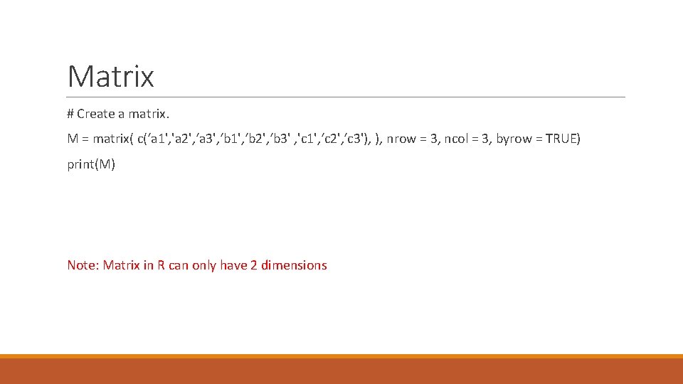
Matrix # Create a matrix. M = matrix( c(‘a 1', 'a 2', ‘a 3', ‘b 1', ‘b 2', ‘b 3' , 'c 1', ‘c 2', ‘c 3'), ), nrow = 3, ncol = 3, byrow = TRUE) print(M) Note: Matrix in R can only have 2 dimensions

Arrays # Create an array. , , 1 a <- array(c(‘heads', ‘tales'), [, 1] dim = c(3, 1, 2)) Print(a) [, 2] [, 3] [1, ] “heads" “tales" “heads" [2, ] “tales" “heads" “tales" [3, ] “heads" “tales" “heads" , , 2 " [, 1] [, 2] [, 3] [1, ] “tales" “heads" “tales" [2, ] “heads" “tales" “heads" [3, ] “tales" “heads" “tales"

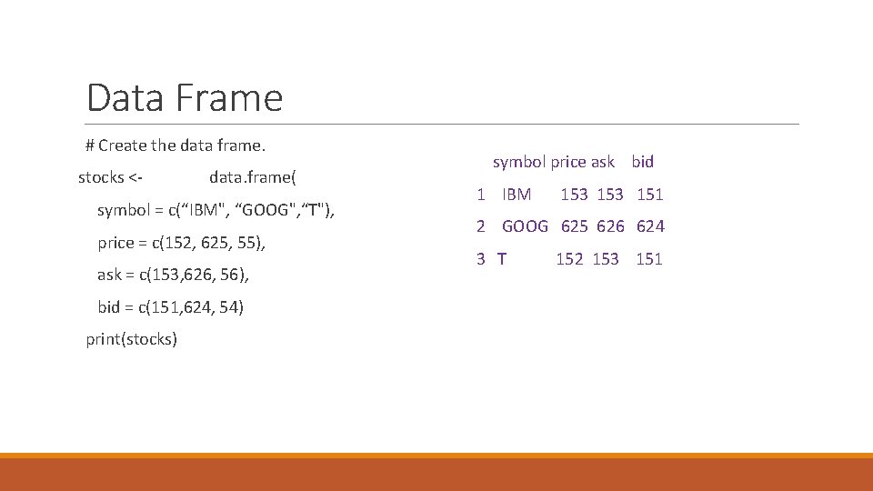
Data Frame # Create the data frame. stocks <- data. frame( symbol = c(“IBM", “GOOG", “T"), price = c(152, 625, 55), ask = c(153, 626, 56), bid = c(151, 624, 54) print(stocks) symbol price ask bid 1 IBM 153 151 2 GOOG 625 626 624 3 T 152 153 151

Factors # Create a vector. sentence <- c(‘me', ‘casa', ‘tu', ‘casa') [1] me casa tu casa # Create a factor object. Levels: me casa tu factor_sentence <- factor(sentence) [1] 3 # Print the factor. print(factor_sentence) print(nlevels(factor_sentence))

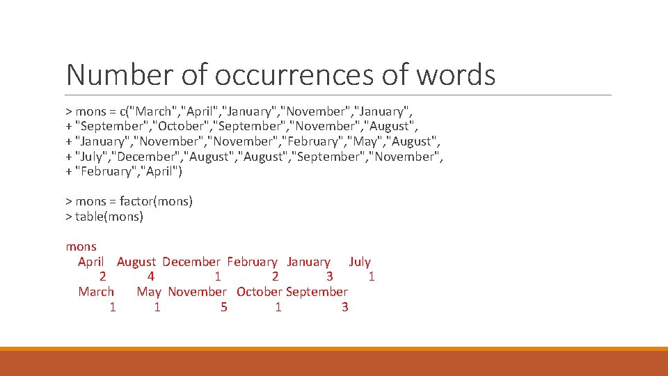
Number of occurrences of words > mons = c("March", "April", "January", "November", "January", + "September", "October", "September", "November", "August", + "January", "November", "February", "May", "August", + "July", "December", "August", "September", "November", + "February", "April") > mons = factor(mons) > table(mons) mons April August December February January July 2 4 1 2 3 1 March May November October September 1 1 5 1 3

Statistics – Mean and standard deviation a <- c(50, 150) mean(a) [1] 100 sd(a) [1] 70. 71068

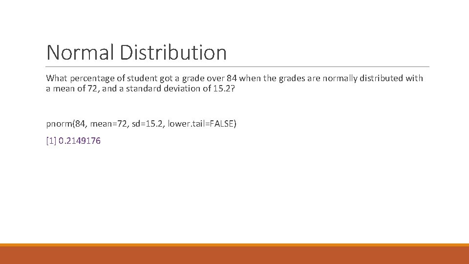
Normal Distribution What percentage of student got a grade over 84 when the grades are normally distributed with a mean of 72, and a standard deviation of 15. 2? pnorm(84, mean=72, sd=15. 2, lower. tail=FALSE) [1] 0. 2149176

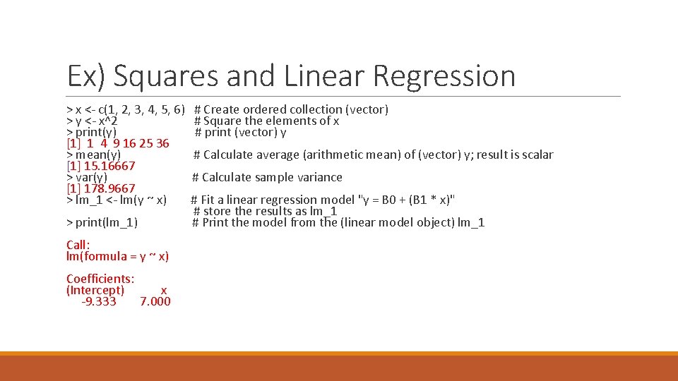
Ex) Squares and Linear Regression > x <- c(1, 2, 3, 4, 5, 6) > y <- x^2 > print(y) [1] 1 4 9 16 25 36 > mean(y) [1] 15. 16667 > var(y) [1] 178. 9667 > lm_1 <- lm(y ~ x) > print(lm_1) Call: lm(formula = y ~ x) Coefficients: (Intercept) x -9. 333 7. 000 # Create ordered collection (vector) # Square the elements of x # print (vector) y # Calculate average (arithmetic mean) of (vector) y; result is scalar # Calculate sample variance # Fit a linear regression model "y = B 0 + (B 1 * x)" # store the results as lm_1 # Print the model from the (linear model object) lm_1

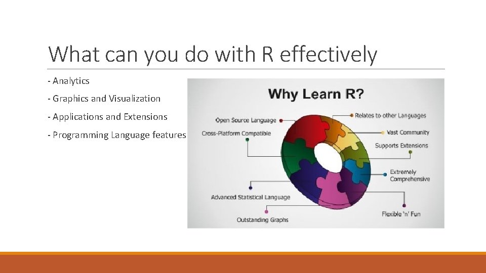
What can you do with R effectively - Analytics - Graphics and Visualization - Applications and Extensions - Programming Language features

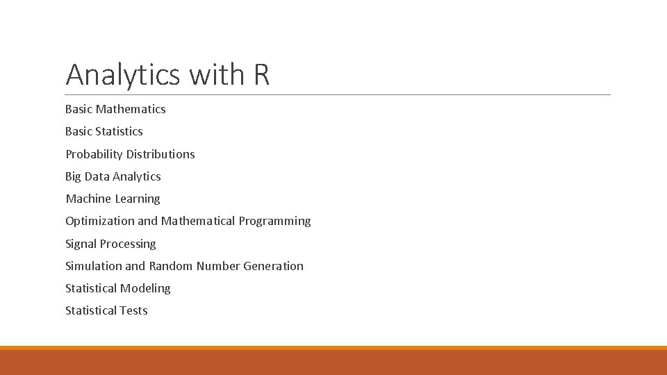
Analytics with R Basic Mathematics Basic Statistics Probability Distributions Big Data Analytics Machine Learning Optimization and Mathematical Programming Signal Processing Simulation and Random Number Generation Statistical Modeling Statistical Tests

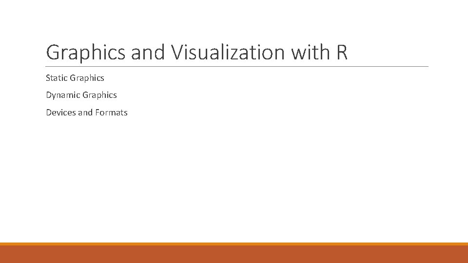
Graphics and Visualization with R Static Graphics Dynamic Graphics Devices and Formats

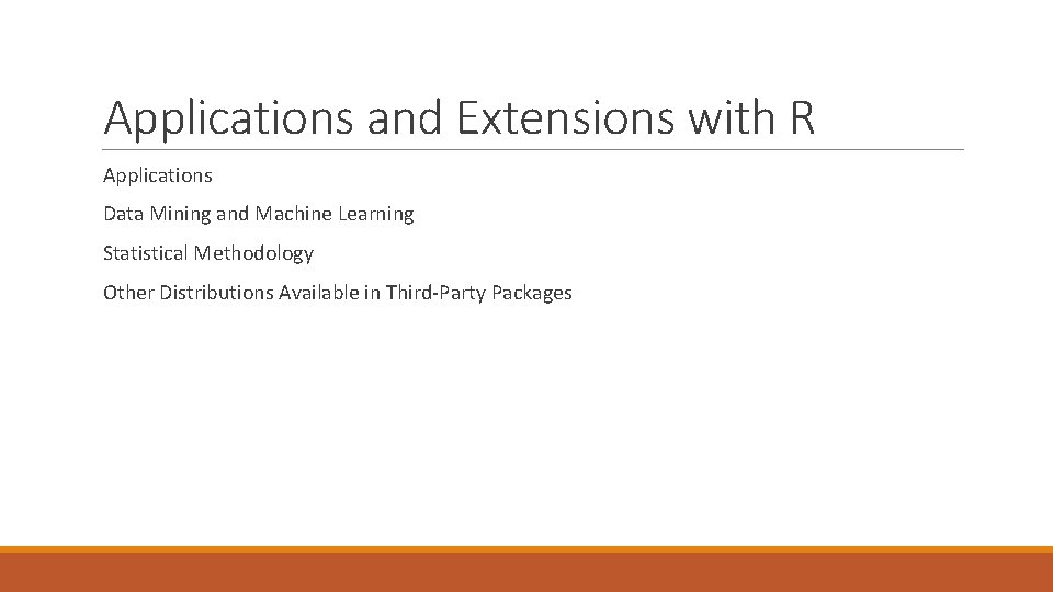
Applications and Extensions with R Applications Data Mining and Machine Learning Statistical Methodology Other Distributions Available in Third-Party Packages

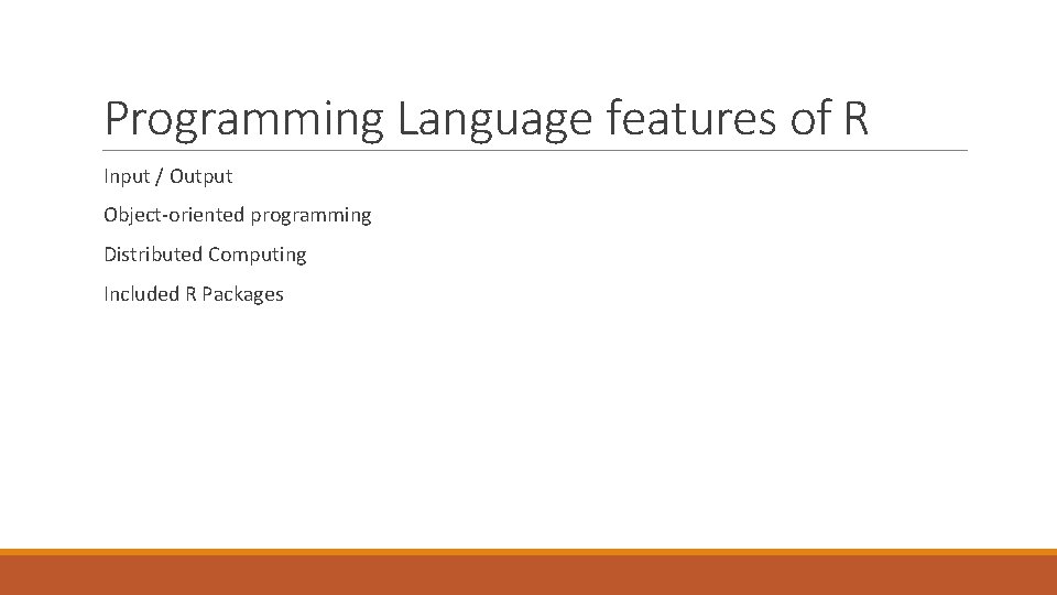
Programming Language features of R Input / Output Object-oriented programming Distributed Computing Included R Packages