R Programming Basics Variables A variable provides us

R- Programming Basics

Variables • A variable provides us with named storage that our programs can manipulate. • A variable in R can store an atomic vector, group of atomic vectors or a combination of many R-objects. • A valid variable name consists of letters, numbers and the dot or underline characters. • The variable name starts with a letter or the dot should not follow by a number.

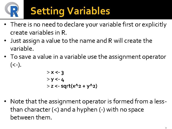
Setting Variables • There is no need to declare your variable first or explicitly create variables in R. • Just assign a value to the name and R will create the variable. • To save a value in a variable use the assignment operator (<-). > x <- 3 > y <- 4 > z <- sqrt(x^2 + y^2) • Note that the assignment operator is formed from a lessthan character (<) and a hyphen (-) with no space between them. 3

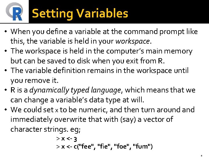
Setting Variables • When you define a variable at the command prompt like this, the variable is held in your workspace. • The workspace is held in the computer’s main memory but can be saved to disk when you exit from R. • The variable definition remains in the workspace until you remove it. • R is a dynamically typed language, which means that we can change a variable’s data type at will. • We could set x to be numeric, and then turn around and immediately overwrite that with (say) a vector of character strings. eg; > x <- 3 > x <- c("fee", "fie", "foe", "fum") 4

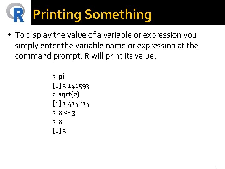
Printing Something • To display the value of a variable or expression you simply enter the variable name or expression at the command prompt, R will print its value. > pi [1] 3. 141593 > sqrt(2) [1] 1. 414214 > x <- 3 >x [1] 3 5

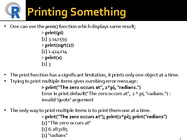
Printing Something • One can use the print() function which displays same result; > print(pi) [1] 3. 141593 > print(sqrt(2)) [1] 1. 414214 > print(x) [1] 3 • The print function has a significant limitation, it prints only one object at a time. • Trying to print multiple items gives numbing error message: > print("The zero occurs at", 2*pi, "radians. ") Error in print. default("The zero occurs at", 2 * pi, "radians. ") : invalid 'quote' argument • The only way to print multiple items is to print them one at a time. > print("The zero occurs at"); print(2*pi); print("radians") [1] "The zero occurs at" [1] 6. 283185 [1] "radians" 6

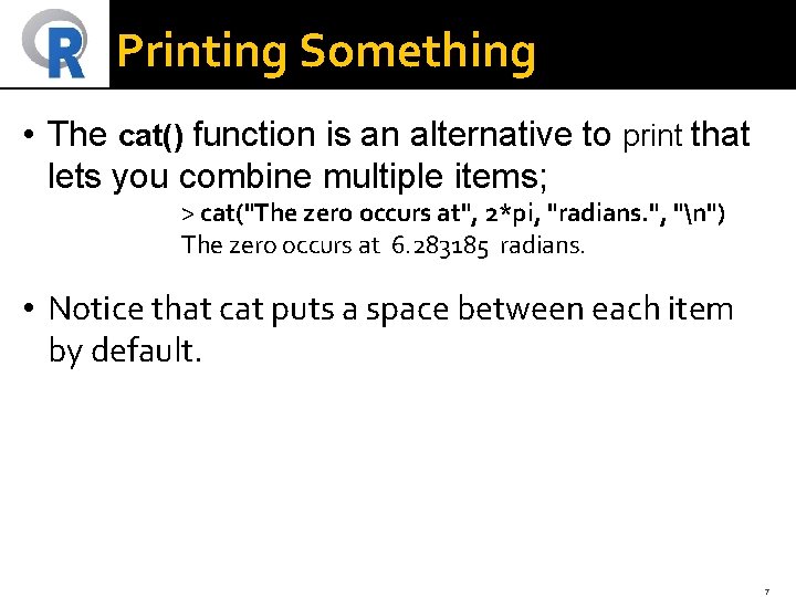
Printing Something • The cat() function is an alternative to print that lets you combine multiple items; > cat("The zero occurs at", 2*pi, "radians. ", "n") The zero occurs at 6. 283185 radians. • Notice that cat puts a space between each item by default. 7

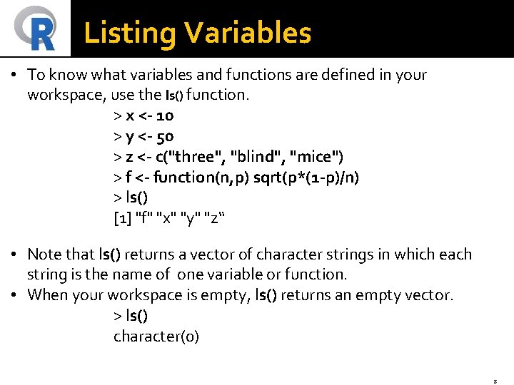
Listing Variables • To know what variables and functions are defined in your workspace, use the ls() function. > x <- 10 > y <- 50 > z <- c("three", "blind", "mice") > f <- function(n, p) sqrt(p*(1 -p)/n) > ls() [1] "f" "x" "y" "z“ • Note that ls() returns a vector of character strings in which each string is the name of one variable or function. • When your workspace is empty, ls() returns an empty vector. > ls() character(0) 8

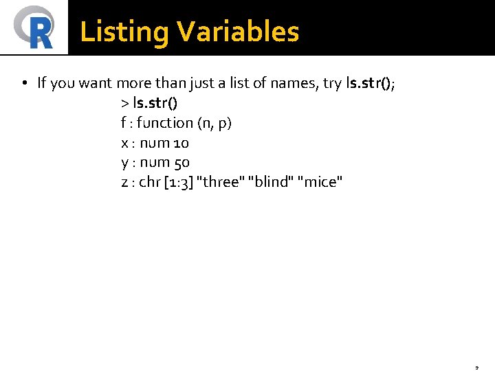
Listing Variables • If you want more than just a list of names, try ls. str(); > ls. str() f : function (n, p) x : num 10 y : num 50 z : chr [1: 3] "three" "blind" "mice" 9

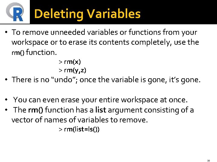
Deleting Variables • To remove unneeded variables or functions from your workspace or to erase its contents completely, use the rm() function. > rm(x) > rm(y, z) • There is no “undo”; once the variable is gone, it’s gone. • You can even erase your entire workspace at once. • The rm() function has a list argument consisting of a vector of names of variables to remove. > rm(list=ls()) 10

R - Operators • An operator is a symbol that tells the compiler to perform specific mathematical or logical manipulations. • R language is rich in built-in operators and provides following types of operators. 11

Types of Operators We have the following types of operators in R programming − • Arithmetic Operators • Relational Operators • Logical Operators 12

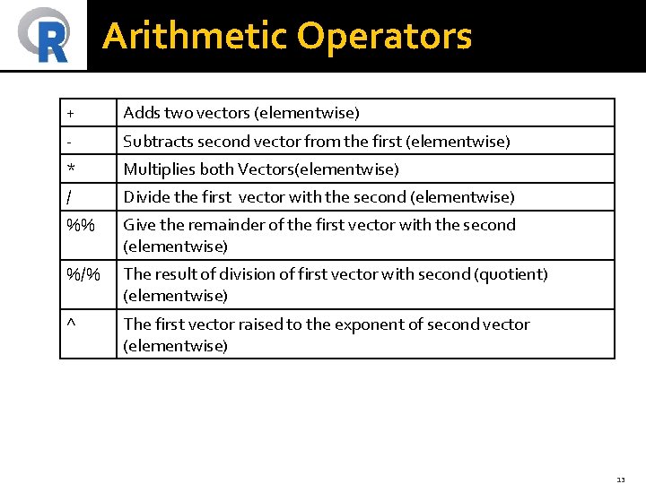
Arithmetic Operators + Adds two vectors (elementwise) - Subtracts second vector from the first (elementwise) * Multiplies both Vectors(elementwise) / Divide the first vector with the second (elementwise) %% Give the remainder of the first vector with the second (elementwise) %/% The result of division of first vector with second (quotient) (elementwise) ^ The first vector raised to the exponent of second vector (elementwise) 13

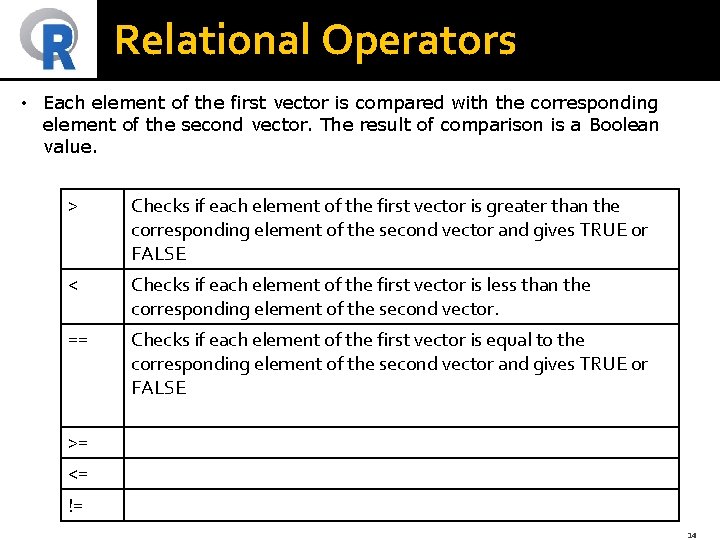
Relational Operators • Each element of the first vector is compared with the corresponding element of the second vector. The result of comparison is a Boolean value. > Checks if each element of the first vector is greater than the corresponding element of the second vector and gives TRUE or FALSE < Checks if each element of the first vector is less than the corresponding element of the second vector. == Checks if each element of the first vector is equal to the corresponding element of the second vector and gives TRUE or FALSE >= <= != 14

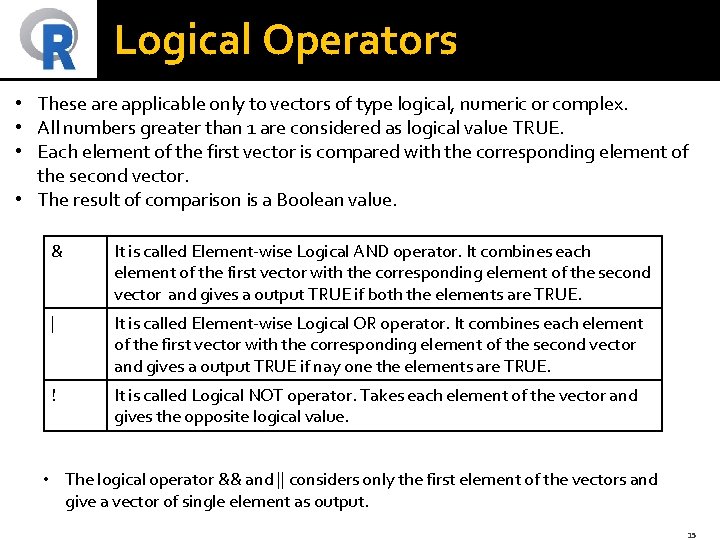
Logical Operators • These are applicable only to vectors of type logical, numeric or complex. • All numbers greater than 1 are considered as logical value TRUE. • Each element of the first vector is compared with the corresponding element of the second vector. • The result of comparison is a Boolean value. & It is called Element-wise Logical AND operator. It combines each element of the first vector with the corresponding element of the second vector and gives a output TRUE if both the elements are TRUE. | It is called Element-wise Logical OR operator. It combines each element of the first vector with the corresponding element of the second vector and gives a output TRUE if nay one the elements are TRUE. ! It is called Logical NOT operator. Takes each element of the vector and gives the opposite logical value. • The logical operator && and || considers only the first element of the vectors and give a vector of single element as output. 15

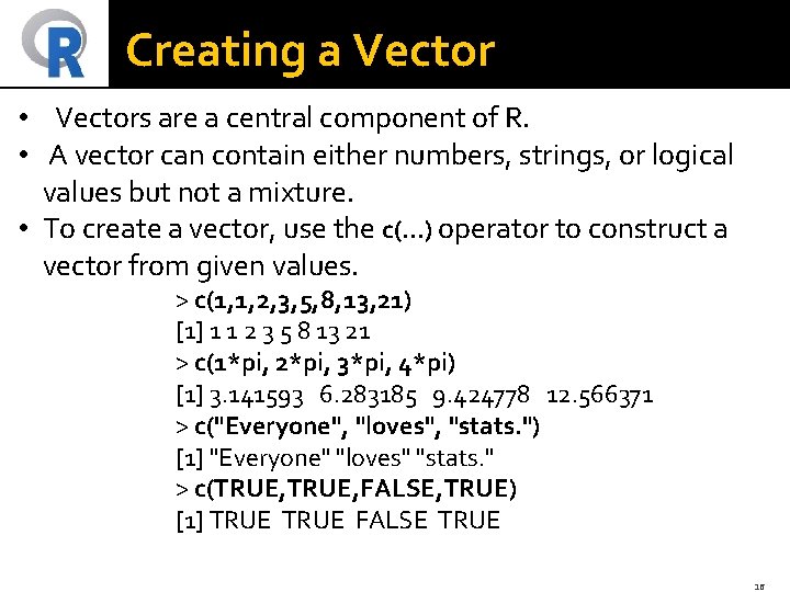
Creating a Vector • Vectors are a central component of R. • A vector can contain either numbers, strings, or logical values but not a mixture. • To create a vector, use the c(. . . ) operator to construct a vector from given values. > c(1, 1, 2, 3, 5, 8, 13, 21) [1] 1 1 2 3 5 8 13 21 > c(1*pi, 2*pi, 3*pi, 4*pi) [1] 3. 141593 6. 283185 9. 424778 12. 566371 > c("Everyone", "loves", "stats. ") [1] "Everyone" "loves" "stats. " > c(TRUE, FALSE, TRUE) [1] TRUE FALSE TRUE 16

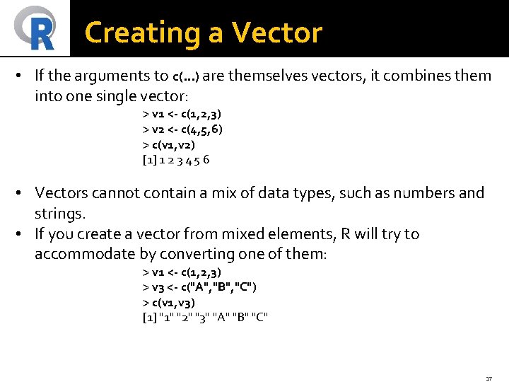
Creating a Vector • If the arguments to c(. . . ) are themselves vectors, it combines them into one single vector: > v 1 <- c(1, 2, 3) > v 2 <- c(4, 5, 6) > c(v 1, v 2) [1] 1 2 3 4 5 6 • Vectors cannot contain a mix of data types, such as numbers and strings. • If you create a vector from mixed elements, R will try to accommodate by converting one of them: > v 1 <- c(1, 2, 3) > v 3 <- c("A", "B", "C") > c(v 1, v 3) [1] "1" "2" "3" "A" "B" "C" 17

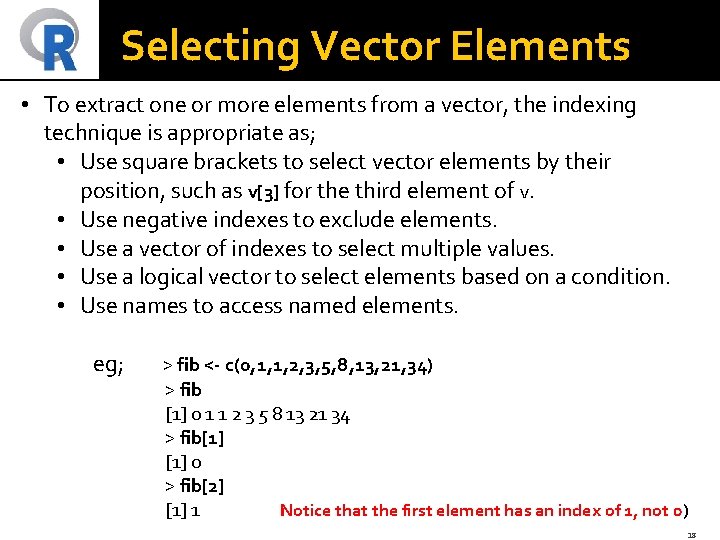
Selecting Vector Elements • To extract one or more elements from a vector, the indexing technique is appropriate as; • Use square brackets to select vector elements by their position, such as v[3] for the third element of v. • Use negative indexes to exclude elements. • Use a vector of indexes to select multiple values. • Use a logical vector to select elements based on a condition. • Use names to access named elements. eg; > fib <- c(0, 1, 1, 2, 3, 5, 8, 13, 21, 34) > fib [1] 0 1 1 2 3 5 8 13 21 34 > fib[1] 0 > fib[2] [1] 1 Notice that the first element has an index of 1, not 0) 18

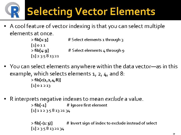
Selecting Vector Elements • A cool feature of vector indexing is that you can select multiple elements at once. > fib[1: 3] [1] 0 1 1 > fib[4: 9] [1] 2 3 5 8 13 21 # Select elements 1 through 3 # Select elements 4 through 9 • You can select elements anywhere within the data vector—as in this example, which selects elements 1, 2, 4, and 8: > fib[c(1, 2, 4, 8)] [1] 0 1 2 13 • R interprets negative indexes to mean exclude a value. > fib[-1] # Ignore first element [1] 1 1 2 3 5 8 13 21 34 > fib[-(1: 3)] # Invert sign of index to exclude instead of select [1] 2 3 5 8 13 21 34 19

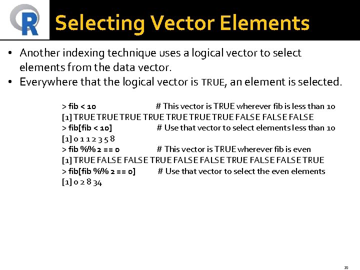
Selecting Vector Elements • Another indexing technique uses a logical vector to select elements from the data vector. • Everywhere that the logical vector is TRUE, an element is selected. > fib < 10 # This vector is TRUE wherever fib is less than 10 [1] TRUE TRUE FALSE > fib[fib < 10] # Use that vector to select elements less than 10 [1] 0 1 1 2 3 5 8 > fib %% 2 == 0 # This vector is TRUE wherever fib is even [1] TRUE FALSE TRUE FALSE TRUE > fib[fib %% 2 == 0] # Use that vector to select the even elements [1] 0 2 8 34 20

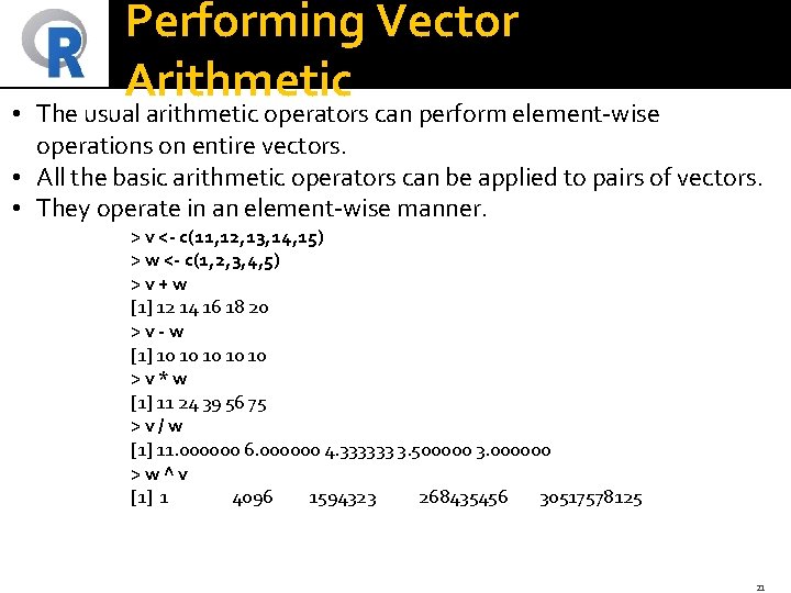
Performing Vector Arithmetic • The usual arithmetic operators can perform element-wise operations on entire vectors. • All the basic arithmetic operators can be applied to pairs of vectors. • They operate in an element-wise manner. > v <- c(11, 12, 13, 14, 15) > w <- c(1, 2, 3, 4, 5) >v+w [1] 12 14 16 18 20 >v-w [1] 10 10 10 >v*w [1] 11 24 39 56 75 >v/w [1] 11. 000000 6. 000000 4. 333333 3. 500000 3. 000000 >w^v [1] 1 4096 1594323 268435456 30517578125 21

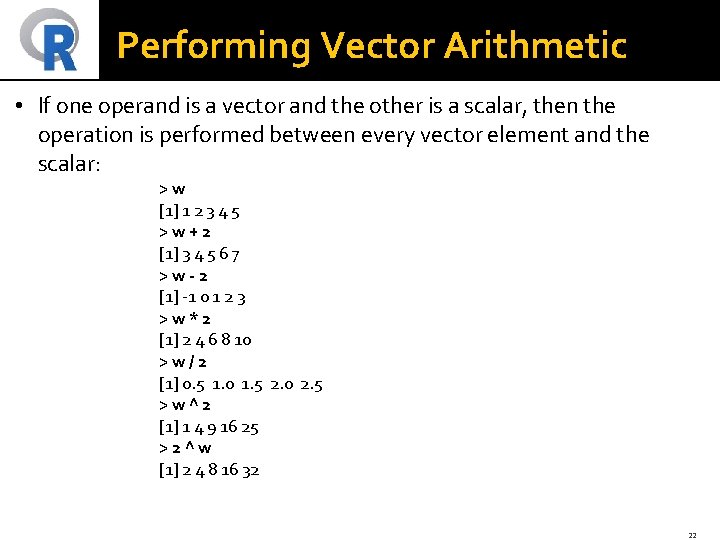
Performing Vector Arithmetic • If one operand is a vector and the other is a scalar, then the operation is performed between every vector element and the scalar: >w [1] 1 2 3 4 5 >w+2 [1] 3 4 5 6 7 >w-2 [1] -1 0 1 2 3 >w*2 [1] 2 4 6 8 10 >w/2 [1] 0. 5 1. 0 1. 5 2. 0 2. 5 >w^2 [1] 1 4 9 16 25 >2^w [1] 2 4 8 16 32 22

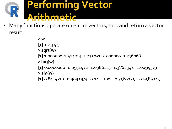
Performing Vector Arithmetic • Many functions operate on entire vectors, too, and return a vector result. >w [1] 1 2 3 4 5 > sqrt(w) [1] 1. 000000 1. 414214 1. 732051 2. 000000 2. 236068 > log(w) [1] 0. 0000000 0. 6931472 1. 0986123 1. 3862944 1. 6094379 > sin(w) [1] 0. 8414710 0. 9092974 0. 1411200 -0. 7568025 -0. 9589243 23

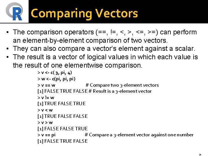
Comparing Vectors • The comparison operators (==, !=, <, >, <=, >=) can perform an element-by-element comparison of two vectors. • They can also compare a vector’s element against a scalar. • The result is a vector of logical values in which each value is the result of one elementwise comparison. > v <- c( 3, pi, 4) > w <- c(pi, pi) > v == w # Compare two 3 -element vectors [1] FALSE TRUE FALSE # Result is a 3 -element vector > v != w [1] TRUE FALSE TRUE >v<w [1] TRUE FALSE >v>w [1] FALSE TRUE > v == pi # Compare a 3 -element vector against one number [1] FALSE TRUE FALSE 24

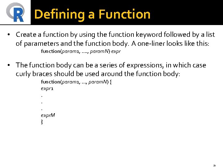
Defining a Function • Create a function by using the function keyword followed by a list of parameters and the function body. A one-liner looks like this: function(param 1, . . , param. N) expr • The function body can be a series of expressions, in which case curly braces should be used around the function body: function(param 1, . . . , param. N) { expr 1. . . expr. M } 25

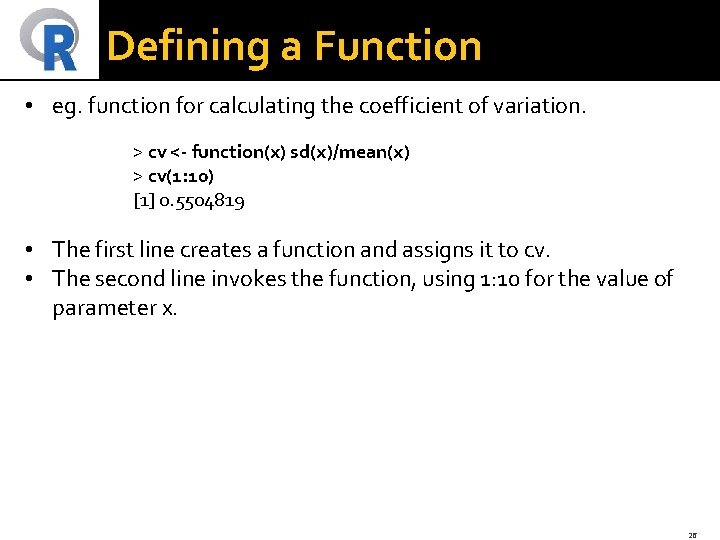
Defining a Function • eg. function for calculating the coefficient of variation. > cv <- function(x) sd(x)/mean(x) > cv(1: 10) [1] 0. 5504819 • The first line creates a function and assigns it to cv. • The second line invokes the function, using 1: 10 for the value of parameter x. 26

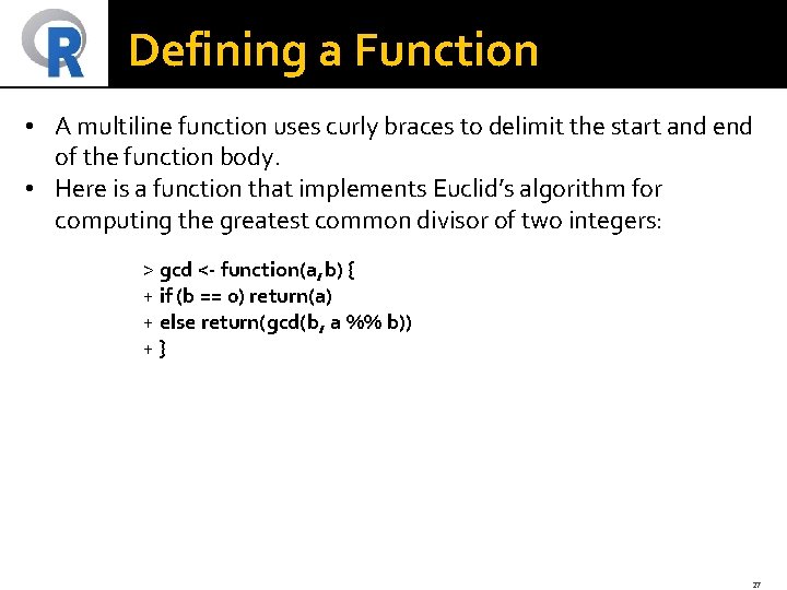
Defining a Function • A multiline function uses curly braces to delimit the start and end of the function body. • Here is a function that implements Euclid’s algorithm for computing the greatest common divisor of two integers: > gcd <- function(a, b) { + if (b == 0) return(a) + else return(gcd(b, a %% b)) +} 27

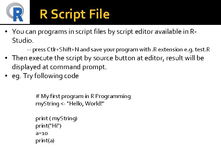
R Script File • You can programs in script files by script editor available in RStudio. -- press Ctlr+Shift+N and save your program with. R extension e. g. test. R • Then execute the script by source button at editor, result will be displayed at command prompt. • eg. Try following code # My first program in R Programming my. String <- "Hello, World!" print ( my. String) print("Hi") a=10 print(a)

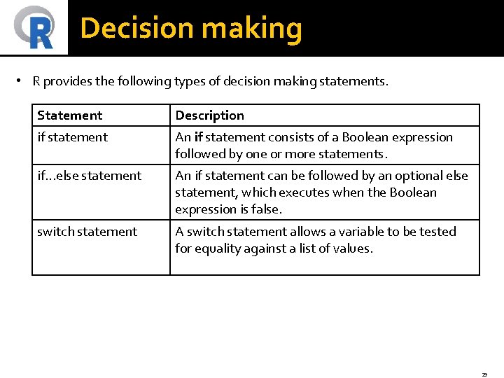
Decision making • R provides the following types of decision making statements. Statement Description if statement An if statement consists of a Boolean expression followed by one or more statements. if. . . else statement An if statement can be followed by an optional else statement, which executes when the Boolean expression is false. switch statement A switch statement allows a variable to be tested for equality against a list of values. 29

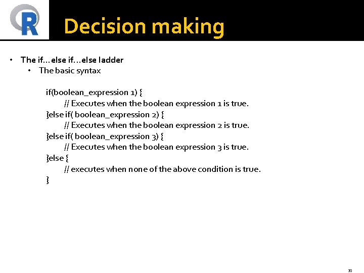
Decision making • The if. . . else ladder • The basic syntax if(boolean_expression 1) { // Executes when the boolean expression 1 is true. }else if( boolean_expression 2) { // Executes when the boolean expression 2 is true. }else if( boolean_expression 3) { // Executes when the boolean expression 3 is true. }else { // executes when none of the above condition is true. } 30

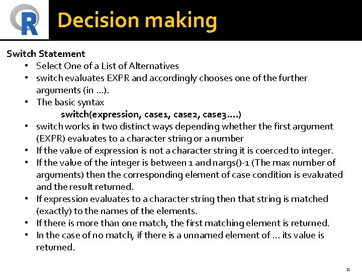
Decision making Switch Statement • Select One of a List of Alternatives • switch evaluates EXPR and accordingly chooses one of the further arguments (in. . . ). • The basic syntax switch(expression, case 1, case 2, case 3. . ) • switch works in two distinct ways depending whether the first argument (EXPR) evaluates to a character string or a number • If the value of expression is not a character string it is coerced to integer. • If the value of the integer is between 1 and nargs()-1 (The max number of arguments) then the corresponding element of case condition is evaluated and the result returned. • If expression evaluates to a character string then that string is matched (exactly) to the names of the elements. • If there is more than one match, the first matching element is returned. • In the case of no match, if there is a unnamed element of. . . its value is returned. 31

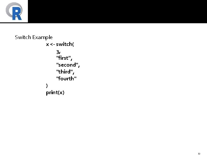
Switch Example x <- switch( 3, "first", "second", "third", "fourth" ) print(x) 32

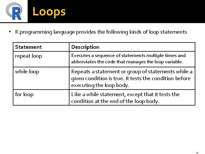
Loops • R programming language provides the following kinds of loop statements Statement Description repeat loop Executes a sequence of statements multiple times and abbreviates the code that manages the loop variable. while loop Repeats a statement or group of statements while a given condition is true. It tests the condition before executing the loop body. for loop Like a while statement, except that it tests the condition at the end of the loop body. 33

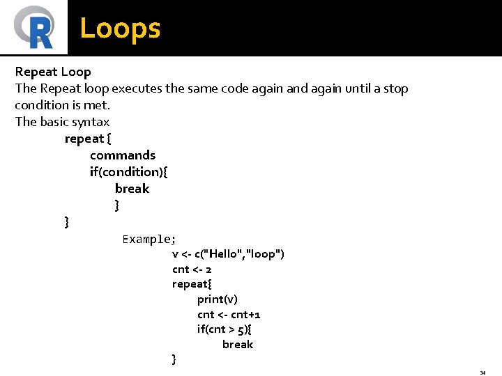
Loops Repeat Loop The Repeat loop executes the same code again and again until a stop condition is met. The basic syntax repeat { commands if(condition){ break } } Example; v <- c("Hello", "loop") cnt <- 2 repeat{ print(v) cnt <- cnt+1 if(cnt > 5){ break } 34

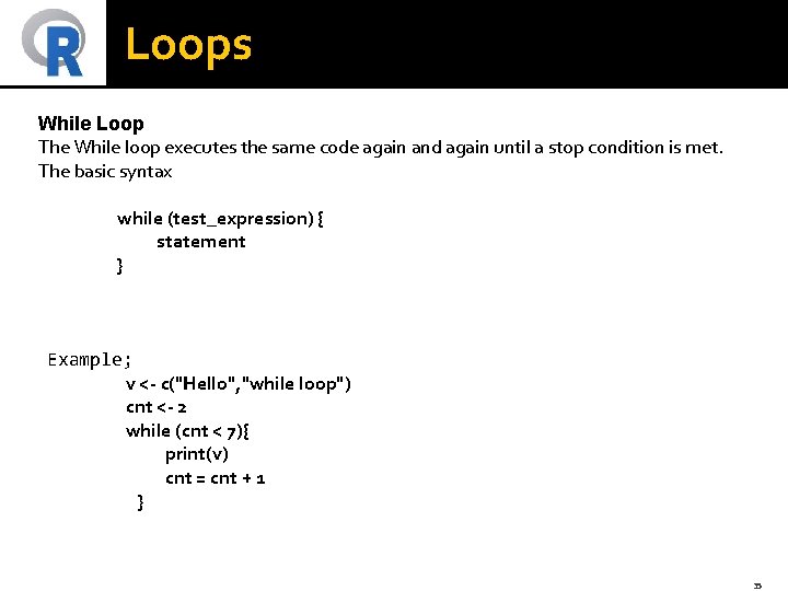
Loops While Loop The While loop executes the same code again and again until a stop condition is met. The basic syntax while (test_expression) { statement } Example; v <- c("Hello", "while loop") cnt <- 2 while (cnt < 7){ print(v) cnt = cnt + 1 } 35

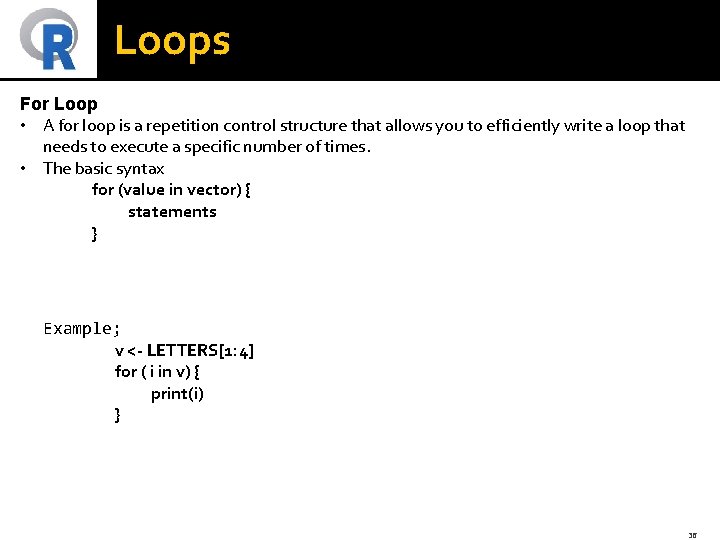
Loops For Loop • A for loop is a repetition control structure that allows you to efficiently write a loop that needs to execute a specific number of times. • The basic syntax for (value in vector) { statements } Example; v <- LETTERS[1: 4] for ( i in v) { print(i) } 36

Thank You 37