R GLENN HUBBARD ANTHONY PATRICK OBRIEN FIFTH EDITION

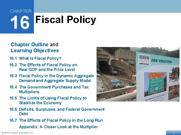
CHAPTER 16 Fiscal Policy Chapter Outline and Learning Objectives 16. 1 What Is Fiscal Policy? 16. 2 The Effects of Fiscal Policy on Real GDP and the Price Level 16. 3 Fiscal Policy in the Dynamic Aggregate Demand Aggregate Supply Model 16. 4 The Government Purchases and Tax Multipliers 16. 5 The Limits of Using Fiscal Policy to Stabilize the Economy 16. 6 Deficits, Surpluses, and Federal Government Debt 16. 7 The Effects of Fiscal Policy in the Long Run Appendix: A Closer Look at the Multiplier © 2015 Pearson Education, Inc. 2

Does Government Spending Create Jobs? Government spending is a component of real GDP: Y = C + I + G + NX This makes it appear as though increases in government spending increase output—and hence other relevant economic variables like employment. However some economists argue that government spending simply shifts employment from one group to another—it does not increase total employment. • This debate was particularly important after the 2007 -2009 recession: can the government use discretionary fiscal policy to increase employment? © 2015 Pearson Education, Inc. 3

What is Fiscal Policy 16. 1 LEARNING OBJECTIVE Define fiscal policy. © 2015 Pearson

Fiscal Policy Defined Fiscal policy refers to changes in federal taxes and purchases that are intended to achieve macroeconomic policy objectives. (State taxes and spending are not generally aimed at affecting national-level objectives. ) Some forms of government spending and taxes automatically increase or decrease along with the business cycle; these are automatic stabilizers. Example: Unemployment insurance payments are larger during a recession. Discretionary fiscal policy, on the other hand, refers to intentional actions the government takes to change spending or taxes. © 2015 Pearson Education, Inc. 5

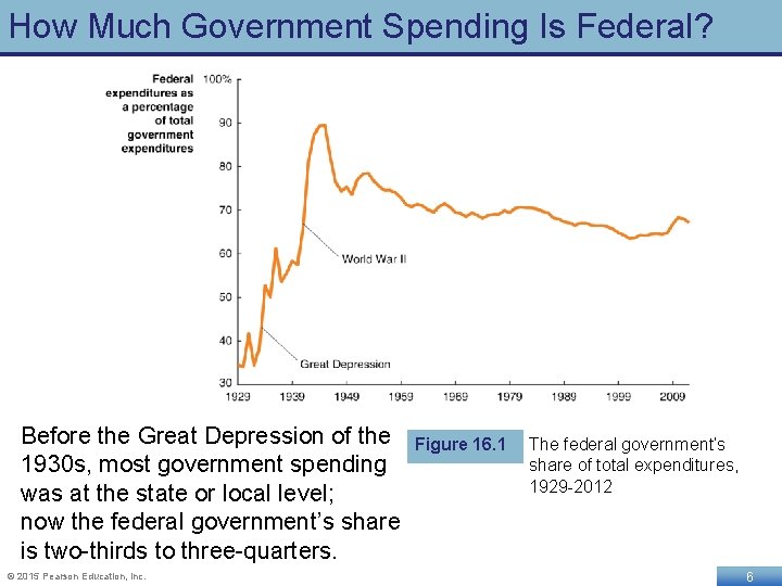
How Much Government Spending Is Federal? Before the Great Depression of the 1930 s, most government spending was at the state or local level; now the federal government’s share is two-thirds to three-quarters. © 2015 Pearson Education, Inc. Figure 16. 1 The federal government’s share of total expenditures, 1929 -2012 6

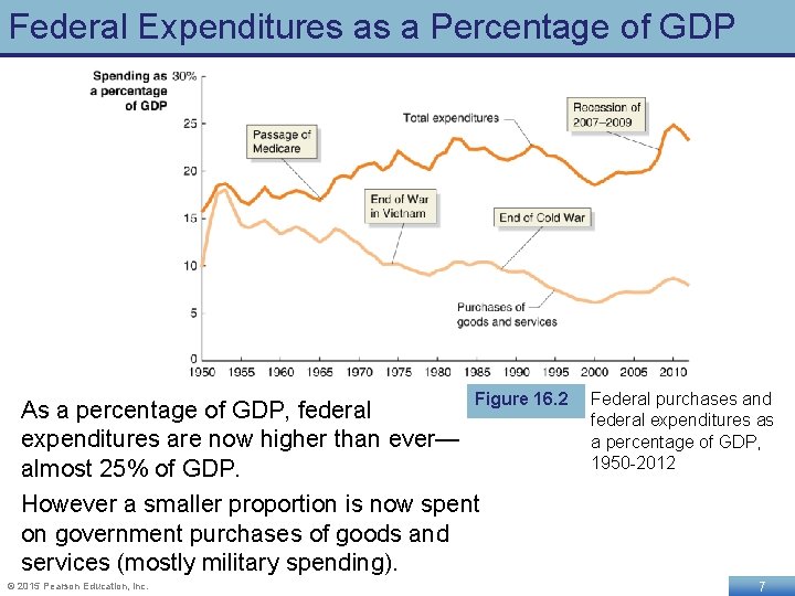
Federal Expenditures as a Percentage of GDP Figure 16. 2 As a percentage of GDP, federal expenditures are now higher than ever— almost 25% of GDP. However a smaller proportion is now spent on government purchases of goods and services (mostly military spending). © 2015 Pearson Education, Inc. Federal purchases and federal expenditures as a percentage of GDP, 1950 -2012 7

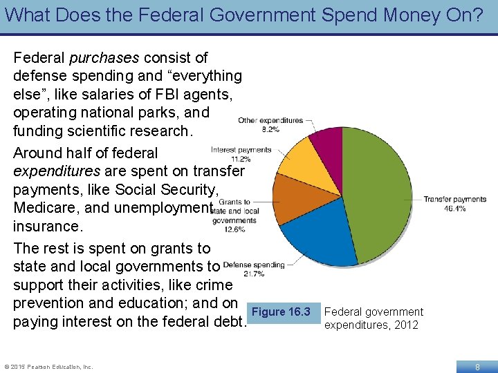
What Does the Federal Government Spend Money On? Federal purchases consist of defense spending and “everything else”, like salaries of FBI agents, operating national parks, and funding scientific research. Around half of federal expenditures are spent on transfer payments, like Social Security, Medicare, and unemployment insurance. The rest is spent on grants to state and local governments to support their activities, like crime prevention and education; and on Figure 16. 3 paying interest on the federal debt. © 2015 Pearson Education, Inc. Federal government expenditures, 2012 8

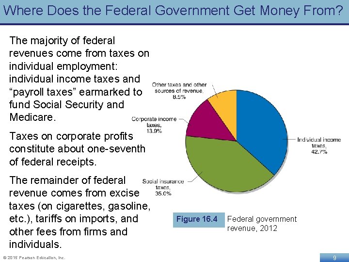
Where Does the Federal Government Get Money From? The majority of federal revenues come from taxes on individual employment: individual income taxes and “payroll taxes” earmarked to fund Social Security and Medicare. Taxes on corporate profits constitute about one-seventh of federal receipts. The remainder of federal revenue comes from excise taxes (on cigarettes, gasoline, etc. ), tariffs on imports, and other fees from firms and individuals. © 2015 Pearson Education, Inc. Figure 16. 4 Federal government revenue, 2012 9

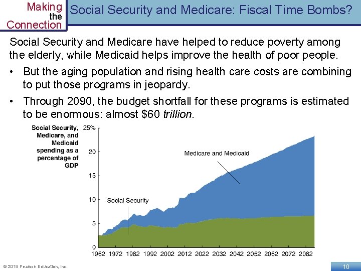
Making Social Security and Medicare: Fiscal Time Bombs? the Connection Social Security and Medicare have helped to reduce poverty among the elderly, while Medicaid helps improve the health of poor people. • But the aging population and rising health care costs are combining to put those programs in jeopardy. • Through 2090, the budget shortfall for these programs is estimated to be enormous: almost $60 trillion. © 2015 Pearson Education, Inc. 10

Making Social Security and Medicare: Is There a Fix? the Connection How can these programs continue to exist? It is likely that a combination of these measures will eventually need to be adopted: • Increasing taxes • Decreasing benefits (including slower benefit growth, perhaps differently for different income groups) • Decreasing eligibility (SSI age already increasing from 65 to 67) But perhaps the most important element will be finding a way to reduce medical costs. © 2015 Pearson Education, Inc. 11

The Effects of Fiscal Policy on Real GDP and the Price Level 16. 2 LEARNING OBJECTIVE Explain how fiscal policy affects aggregate demand how the government can use fiscal policy to stabilize the economy. © 2015 Pearson Education, Inc. 12

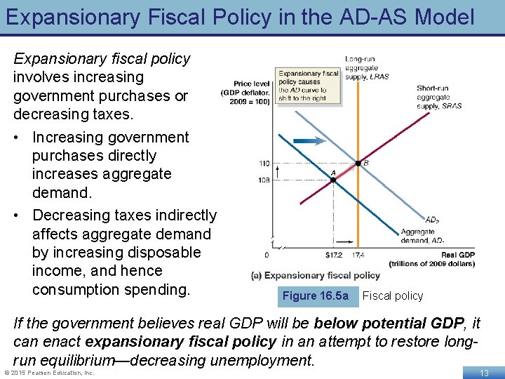
Expansionary Fiscal Policy in the AD-AS Model Expansionary fiscal policy involves increasing government purchases or decreasing taxes. • Increasing government purchases directly increases aggregate demand. • Decreasing taxes indirectly affects aggregate demand by increasing disposable income, and hence consumption spending. Figure 16. 5 a Fiscal policy If the government believes real GDP will be below potential GDP, it can enact expansionary fiscal policy in an attempt to restore longrun equilibrium—decreasing unemployment. © 2015 Pearson Education, Inc. 13

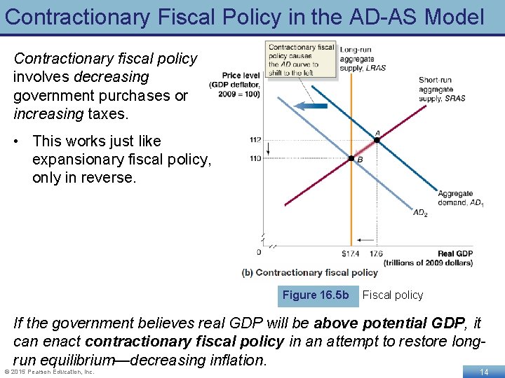
Contractionary Fiscal Policy in the AD-AS Model Contractionary fiscal policy involves decreasing government purchases or increasing taxes. • This works just like expansionary fiscal policy, only in reverse. Figure 16. 5 b Fiscal policy If the government believes real GDP will be above potential GDP, it can enact contractionary fiscal policy in an attempt to restore longrun equilibrium—decreasing inflation. © 2015 Pearson Education, Inc. 14

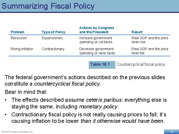
Summarizing Fiscal Policy Actions by Congress and the President Result Problem Type of Policy Recession Expansionary Increase government spending or cut taxes Real GDP and the price level rise. Rising inflation Contractionary Decrease government spending or raise taxes Real GDP and the price level fall. Table 16. 1 Countercyclical fiscal policy The federal government’s actions described on the previous slides constitute a countercyclical fiscal policy. Bear in mind that: • The effects described assume ceteris paribus: everything else is staying the same, including monetary policy. • Contractionary fiscal policy is not really causing prices to fall; it’s causing inflation to be lower than it otherwise would have been. © 2015 Pearson Education, Inc. 15

Fiscal Policy in the Dynamic Aggregate Demand Aggregate Supply Model 16. 3 LEARNING OBJECTIVE Use the dynamic aggregate demand aggregate supply model to analyze fiscal policy. © 2015 Pearson Education, Inc. 16

Static vs. Dynamic Model Our model of fiscal policy so far is static: it assumes long-run potential GDP does not change, and that the price level is constant. While the lessons from this model are still appropriate—Congress and the president can use fiscal policy to affect real GDP and the price level—our understanding of fiscal policy can be improved by seeing it in the dynamic aggregate demand aggregate supply model. © 2015 Pearson Education, Inc. 17

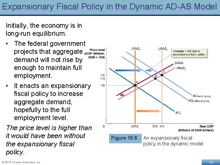
Expansionary Fiscal Policy in the Dynamic AD-AS Model Initially, the economy is in long-run equilibrium. • The federal government projects that aggregate demand will not rise by enough to maintain full employment. • It enacts an expansionary fiscal policy to increase aggregate demand, hopefully to the full employment level. The price level is higher than it would have been without the expansionary fiscal policy. © 2015 Pearson Education, Inc. Figure 16. 6 An expansionary fiscal policy in the dynamic model 18

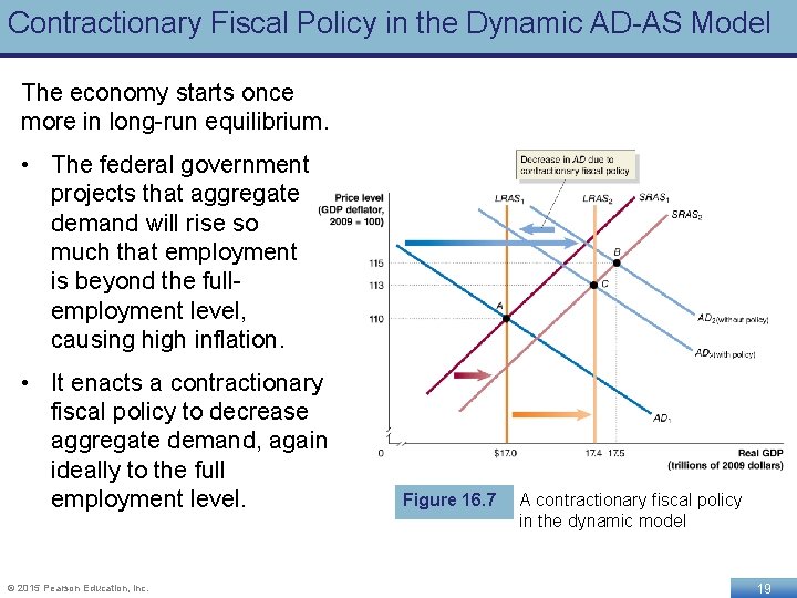
Contractionary Fiscal Policy in the Dynamic AD-AS Model The economy starts once more in long-run equilibrium. • The federal government projects that aggregate demand will rise so much that employment is beyond the fullemployment level, causing high inflation. • It enacts a contractionary fiscal policy to decrease aggregate demand, again ideally to the full employment level. © 2015 Pearson Education, Inc. Figure 16. 7 A contractionary fiscal policy in the dynamic model 19

The Government Purchases and Tax Multipliers 16. 4 LEARNING OBJECTIVE Explain how the government

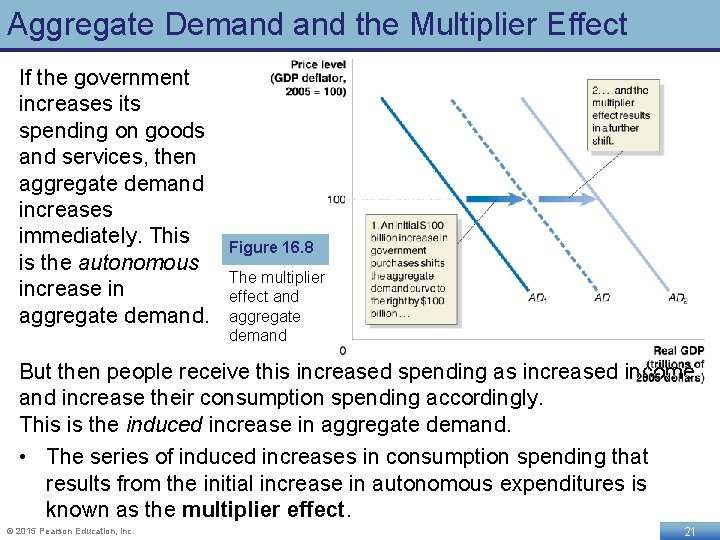
Aggregate Demand the Multiplier Effect If the government increases its spending on goods and services, then aggregate demand increases immediately. This is the autonomous increase in aggregate demand. Figure 16. 8 The multiplier effect and aggregate demand But then people receive this increased spending as increased income and increase their consumption spending accordingly. This is the induced increase in aggregate demand. • The series of induced increases in consumption spending that results from the initial increase in autonomous expenditures is known as the multiplier effect. © 2015 Pearson Education, Inc. 21

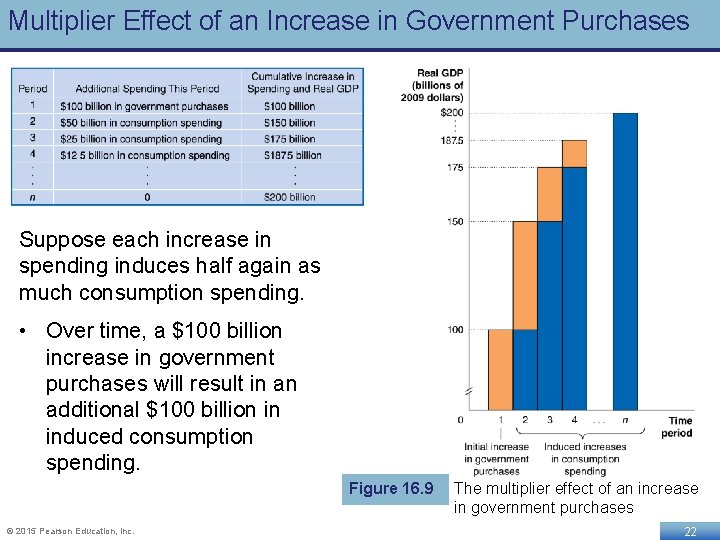
Multiplier Effect of an Increase in Government Purchases Suppose each increase in spending induces half again as much consumption spending. • Over time, a $100 billion increase in government purchases will result in an additional $100 billion in induced consumption spending. Figure 16. 9 © 2015 Pearson Education, Inc. The multiplier effect of an increase in government purchases 22

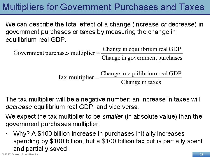
Multipliers for Government Purchases and Taxes We can describe the total effect of a change (increase or decrease) in government purchases or taxes by measuring the change in equilibrium real GDP. The tax multiplier will be a negative number: an increase in taxes will decrease equilibrium real GDP, and vice versa. We expect the tax multiplier to be smaller (in absolute value) than the government purchases multiplier. • Why? A $100 billion increase in purchases initially increases spending by $100 billion, but a $100 billion tax cut is partially spent and partially saved. © 2015 Pearson Education, Inc. 23

The Effect of Changes in Tax Rates The tax multiplier applies to changes in the amount of taxes, without changes in tax rates. Example: In 2009 and 2010, the federal government enacted the Making Work Pay Tax Credit: a $400 reduction in taxes for working individuals ($800 for households). Decreases in tax rates have a slightly different effect: 1. Increasing the disposable income of households, leading them to increase their consumption spending. 2. Increasing the size of the multiplier effect, since more of any increase in income becomes disposable income. © 2015 Pearson Education, Inc. 24

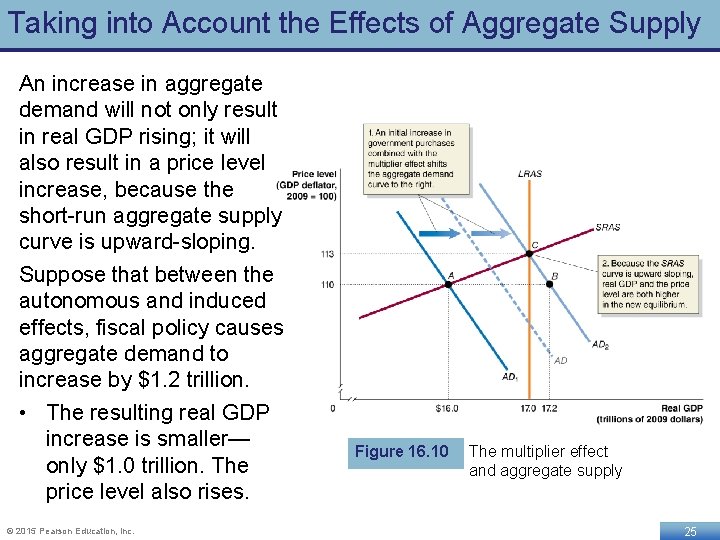
Taking into Account the Effects of Aggregate Supply An increase in aggregate demand will not only result in real GDP rising; it will also result in a price level increase, because the short-run aggregate supply curve is upward-sloping. Suppose that between the autonomous and induced effects, fiscal policy causes aggregate demand to increase by $1. 2 trillion. • The resulting real GDP increase is smaller— only $1. 0 trillion. The price level also rises. © 2015 Pearson Education, Inc. Figure 16. 10 The multiplier effect and aggregate supply 25

The Multipliers Work in Both Directions An increase in government purchases and a cut in taxes have a positive multiplier effect. A decrease in government purchases and an increase in taxes have a negative multiplier effect. Example: a reduction in government spending on defense initially affects defense contractors, but then it would spread to suppliers to and employees of those contractors, and then to other firms and workers. © 2015 Pearson Education, Inc. 26

The Limits of Using Fiscal Policy to Stabilize the Economy 16. 5 LEARNING OBJECTIVE

Can We Use Fiscal Policy to Stabilize the Economy? For several reasons, fiscal policy may be even less effective than monetary policy at countercyclical stabilization: • Timing fiscal policy is harder, due to: • Legislative delay: Congress needs to agree on the actions • Implementation delay: Large spending projects may take months or even years to begin, even once approved. • Government spending might crowd out private spending Crowding out: A decline in private expenditures as a result of an increase in government purchases © 2015 Pearson Education, Inc. 28

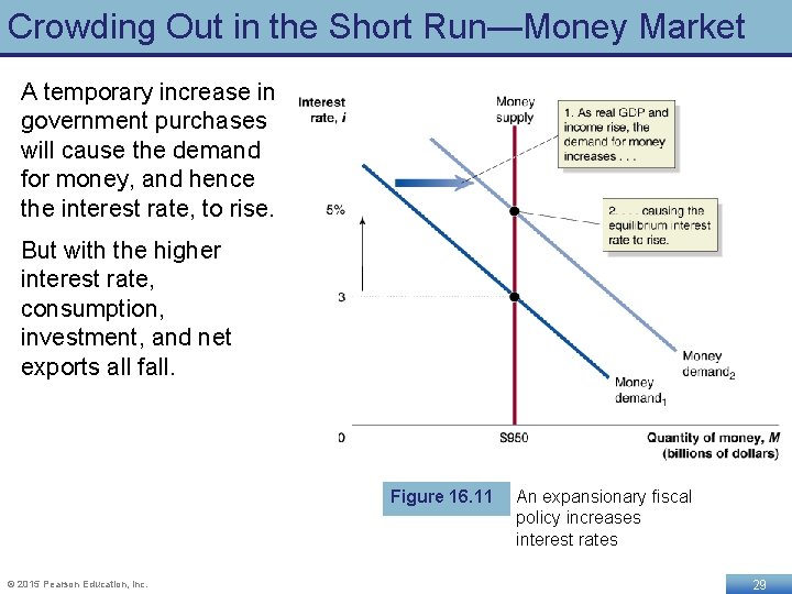
Crowding Out in the Short Run—Money Market A temporary increase in government purchases will cause the demand for money, and hence the interest rate, to rise. But with the higher interest rate, consumption, investment, and net exports all fall. Figure 16. 11 © 2015 Pearson Education, Inc. An expansionary fiscal policy increases interest rates 29

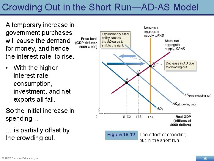
Crowding Out in the Short Run—AD-AS Model A temporary increase in government purchases will cause the demand for money, and hence the interest rate, to rise. • With the higher interest rate, consumption, investment, and net exports all fall. So the initial increase in spending… … is partially offset by the crowding out. © 2015 Pearson Education, Inc. Figure 16. 12 The effect of crowding out in the short run 30

Crowding Out in the Long Run In the long run, the increase in government purchases will have no effect on real GDP; the reduction in consumption, investment, and net exports will exactly offset the increase in government purchases. • Why? Because in the long run, the economy returns to potential GDP, even without the government’s intervention. The long run effect is simply to increase the size of the government sector within the economy. • Bear in mind that the long run may be many years away, however, so the intermediate increase in real GDP may be worth the cost. © 2015 Pearson Education, Inc. 31

Fiscal Policy in Action: The 2007 -2009 Recession In early 2008, believing a recession was imminent, Congress authorized a tax cut: a one-time rebate of taxes already paid, totaling $95 billion. • This resulted in a boost to consumers’ current incomes. Changes to current incomes result in smaller increases in spending than changes to permanent incomes, because people seek to “smooth” their consumption over time. • Economists estimate that consumers spent about 33 -40% of the rebates they received, so the tax cut resulted in about $35 billion in increased spending. © 2015 Pearson Education, Inc. 32

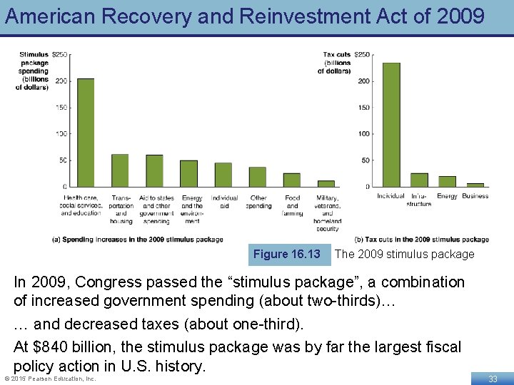
American Recovery and Reinvestment Act of 2009 Figure 16. 13 The 2009 stimulus package In 2009, Congress passed the “stimulus package”, a combination of increased government spending (about two-thirds)… … and decreased taxes (about one-third). At $840 billion, the stimulus package was by far the largest fiscal policy action in U. S. history. © 2015 Pearson Education, Inc. 33

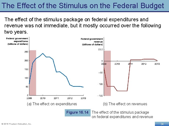
The Effect of the Stimulus on the Federal Budget The effect of the stimulus package on federal expenditures and revenue was not immediate, but it mostly occurred over the following two years. (a) The effect on expenditures (b) The effect on revenues Figure 16. 14 The effect of the stimulus package on federal expenditures and revenue © 2015 Pearson Education, Inc. 34

How Effective Was the Stimulus Package? When the stimulus was passed, Obama administration economists believed that by the end of 2010, it would: • Increase real GDP by 3. 5% • Increase employment by 3. 5 million By the end of 2010, real GDP actually rose by 4. 4% but employment fell by 3. 3 million. Did the stimulus fail? • To judge the effect of the stimulus package, we have to measure its effects holding constant all other factors affecting real GDP and employment. • Isolating the effects of the stimulus package is very difficult; economists still differ in their views about how effective the stimulus package was. © 2015 Pearson Education, Inc. 35

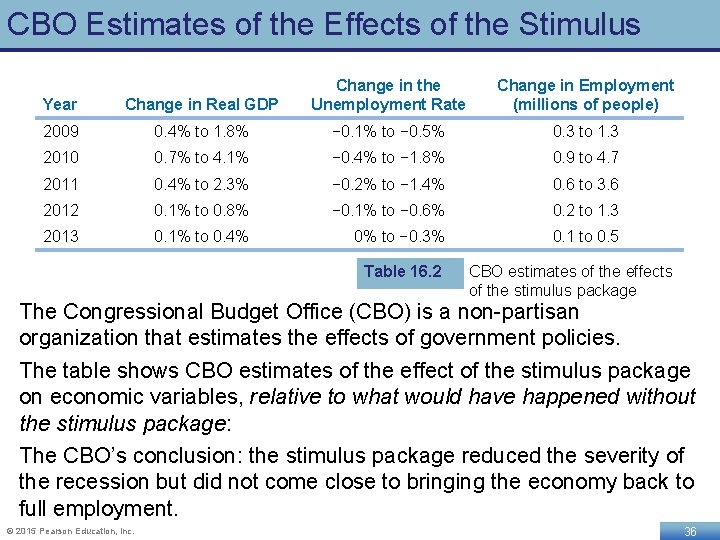
CBO Estimates of the Effects of the Stimulus Year Change in Real GDP Change in the Unemployment Rate 2009 0. 4% to 1. 8% − 0. 1% to − 0. 5% 0. 3 to 1. 3 2010 0. 7% to 4. 1% − 0. 4% to − 1. 8% 0. 9 to 4. 7 2011 0. 4% to 2. 3% − 0. 2% to − 1. 4% 0. 6 to 3. 6 2012 0. 1% to 0. 8% − 0. 1% to − 0. 6% 0. 2 to 1. 3 2013 0. 1% to 0. 4% 0% to − 0. 3% 0. 1 to 0. 5 Table 16. 2 Change in Employment (millions of people) CBO estimates of the effects of the stimulus package The Congressional Budget Office (CBO) is a non-partisan organization that estimates the effects of government policies. The table shows CBO estimates of the effect of the stimulus package on economic variables, relative to what would have happened without the stimulus package: The CBO’s conclusion: the stimulus package reduced the severity of the recession but did not come close to bringing the economy back to full employment. © 2015 Pearson Education, Inc. 36

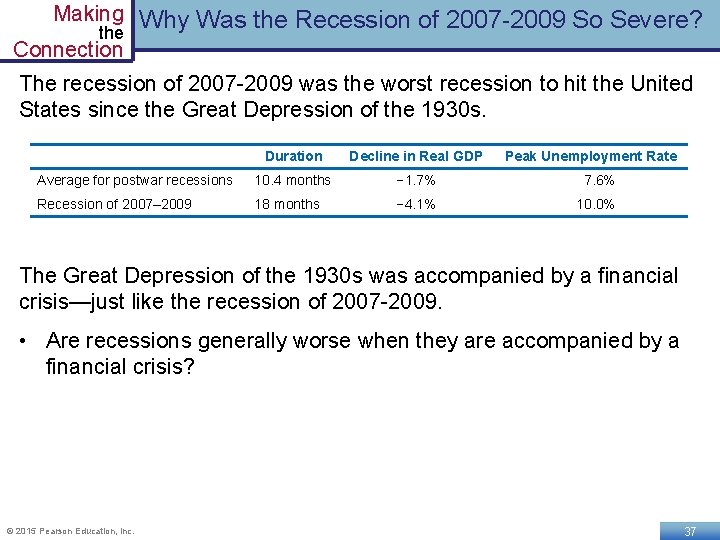
Making Why Was the Recession of 2007 -2009 So Severe? the Connection The recession of 2007 -2009 was the worst recession to hit the United States since the Great Depression of the 1930 s. Duration Decline in Real GDP Peak Unemployment Rate Average for postwar recessions 10. 4 months − 1. 7% 7. 6% Recession of 2007– 2009 18 months − 4. 1% 10. 0% The Great Depression of the 1930 s was accompanied by a financial crisis—just like the recession of 2007 -2009. • Are recessions generally worse when they are accompanied by a financial crisis? © 2015 Pearson Education, Inc. 37

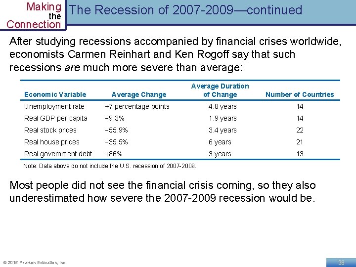
Making The Recession of 2007 -2009—continued the Connection After studying recessions accompanied by financial crises worldwide, economists Carmen Reinhart and Ken Rogoff say that such recessions are much more severe than average: Average Duration of Change Economic Variable Average Change Number of Countries Unemployment rate +7 percentage points 4. 8 years 14 Real GDP per capita − 9. 3% 1. 9 years 14 Real stock prices − 55. 9% 3. 4 years 22 Real house prices − 35. 5% 6 years 21 Real government debt +86% 3 years 13 Note: Data above do not include the U. S. recession of 2007 -2009. Most people did not see the financial crisis coming, so they also underestimated how severe the 2007 -2009 recession would be. © 2015 Pearson Education, Inc. 38

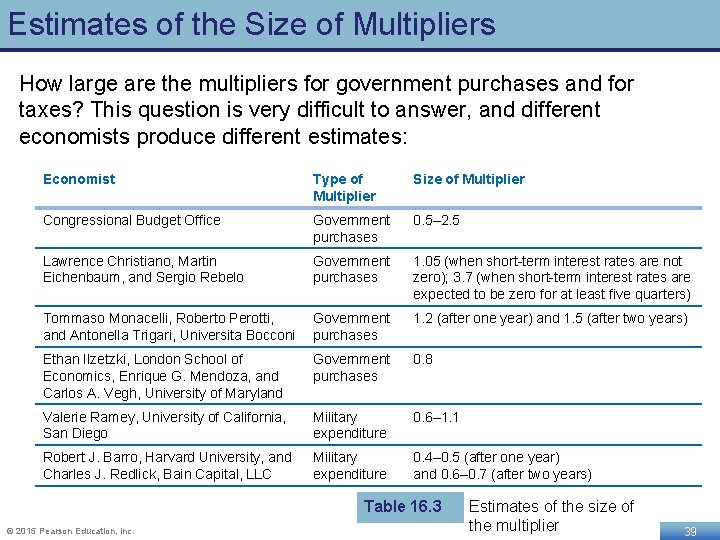
Estimates of the Size of Multipliers How large are the multipliers for government purchases and for taxes? This question is very difficult to answer, and different economists produce different estimates: Economist Type of Multiplier Size of Multiplier Congressional Budget Office Government purchases 0. 5– 2. 5 Lawrence Christiano, Martin Eichenbaum, and Sergio Rebelo Government purchases 1. 05 (when short-term interest rates are not zero); 3. 7 (when short-term interest rates are expected to be zero for at least five quarters) Tommaso Monacelli, Roberto Perotti, and Antonella Trigari, Universita Bocconi Government purchases 1. 2 (after one year) and 1. 5 (after two years) Ethan Ilzetzki, London School of Economics, Enrique G. Mendoza, and Carlos A. Vegh, University of Maryland Government purchases 0. 8 Valerie Ramey, University of California, San Diego Military expenditure 0. 6– 1. 1 Robert J. Barro, Harvard University, and Charles J. Redlick, Bain Capital, LLC Military expenditure 0. 4– 0. 5 (after one year) and 0. 6– 0. 7 (after two years) Table 16. 3 © 2015 Pearson Education, Inc. Estimates of the size of the multiplier 39

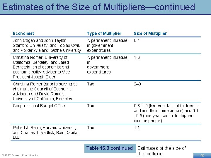
Estimates of the Size of Multipliers—continued Economist Type of Multiplier Size of Multiplier John Cogan and John Taylor, Stanford University, and Tobias Cwik and Volker Wieland, Gothe University A permanent increase in government expenditures 0. 4 Christina Romer, University of California, Berkeley, and Jared Bernstein, chief economist and economic policy adviser to Vice President Joseph Biden A permanent increase in government expenditures 1. 6 Christina Romer (prior to serving as chair of the Council of Economic Advisers) and David Romer, University of California, Berkeley Tax 2– 3 Congressional Budget Office Tax 0. 6– 1. 5 (two-year tax cut for lowerand middle-income people) and 0. 1 – 0. 6 (one-year tax cut for higherincome people) Robert J. Barro, Harvard University, and Charles J. Redlick, Bain Capital, LLC Tax 1. 1 © 2015 Pearson Education, Inc. Table 16. 3 continued Estimates of the size of the multiplier 40

Deficits, Surpluses, and Federal Government Debt 16. 6 LEARNING OBJECTIVE Define federal budget deficit and federal government debt, and explain how the federal budget can serve as an automatic stabilizer. © 2015 Pearson Education, Inc. 41

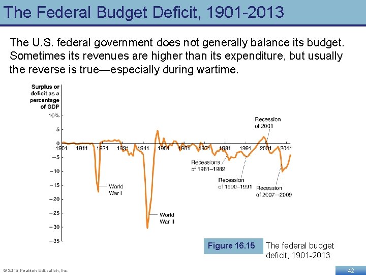
The Federal Budget Deficit, 1901 -2013 The U. S. federal government does not generally balance its budget. Sometimes its revenues are higher than its expenditure, but usually the reverse is true—especially during wartime. Figure 16. 15 © 2015 Pearson Education, Inc. The federal budget deficit, 1901 -2013 42

Budget Deficits and Surpluses A budget deficit occurs when the government’s expenditures are greater than its tax revenue. A budget surplus occurs when the government’s expenditures are less than its tax revenue. As the graph on the previous slide indicates, budget deficits often occur during wartime. • But they also occur during recessions, as tax receipts fall, and automatic stabilizers like increases in transfer payments (unemployment insurance, food stamps, etc. ) take effect. • These automatic stabilizers are important for limiting the severity of a recession; many economists believe that the Great Depression of the 1930 s was more severe because most of these automatic stabilizers did not exist then. © 2015 Pearson Education, Inc. 43

How Large Is the Deficit in the United States? Currently, the federal government runs a budget deficit; the CBO estimated in 2013 that the deficit for 2014 would be about 3. 5% of real GDP. • How much of this deficit is due to the recession, and how much is due to government spending and tax policies? We can identify this by looking at the cyclically adjusted budget deficit or surplus: the deficit or surplus in the federal government’s budget if the economy were at potential GDP. • The CBO estimated that the budget deficit would be 1. 0% of real GDP in 2014 if real GDP were at its potential. • So this is the amount that spending needs to be cut, or taxes raised, in order to bring the federal budget into balance in the long run. The rest is due to automatic stabilizers. © 2015 Pearson Education, Inc. 44

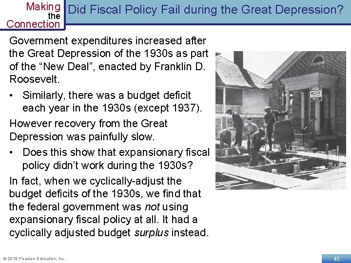
Making Did Fiscal Policy Fail during the Great Depression? the Connection Government expenditures increased after the Great Depression of the 1930 s as part of the “New Deal”, enacted by Franklin D. Roosevelt. • Similarly, there was a budget deficit each year in the 1930 s (except 1937). However recovery from the Great Depression was painfully slow. • Does this show that expansionary fiscal policy didn’t work during the 1930 s? In fact, when we cyclically-adjust the budget deficits of the 1930 s, we find that the federal government was not using expansionary fiscal policy at all. It had a cyclically adjusted budget surplus instead. © 2015 Pearson Education, Inc. 45

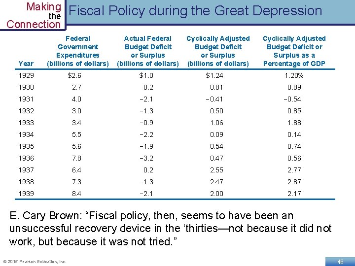
Making the Fiscal Policy during the Great Depression Connection Year Federal Government Expenditures (billions of dollars) Actual Federal Budget Deficit or Surplus (billions of dollars) Cyclically Adjusted Budget Deficit or Surplus as a Percentage of GDP 1929 $2. 6 $1. 0 $1. 24 1. 20% 1930 2. 7 0. 2 0. 81 0. 89 1931 4. 0 − 2. 1 − 0. 41 − 0. 54 1932 3. 0 − 1. 3 0. 50 0. 85 1933 3. 4 − 0. 9 1. 06 1. 88 1934 5. 5 − 2. 2 0. 09 0. 14 1935 5. 6 − 1. 9 0. 54 0. 74 1936 7. 8 − 3. 2 0. 47 0. 56 1937 6. 4 0. 2 2. 55 2. 77 1938 7. 3 − 1. 3 2. 47 2. 87 1939 8. 4 − 2. 1 2. 00 2. 17 E. Cary Brown: “Fiscal policy, then, seems to have been an unsuccessful recovery device in the ‘thirties—not because it did not work, but because it was not tried. ” © 2015 Pearson Education, Inc. 46

Should the Federal Budget Always Be Balanced? Although many economists believe the federal budget should be balanced when the economy is at potential GDP, few believe it should be balanced during a recession. • During a recession, tax revenues fall; to balance the budget, spending would have to fall also—making the recession worse. In fact, some economists argue that the federal budget should normally be in deficit. Just as households and firms borrow money to implement long-term investments, they argue that the federal government should do the same. © 2015 Pearson Education, Inc. 47

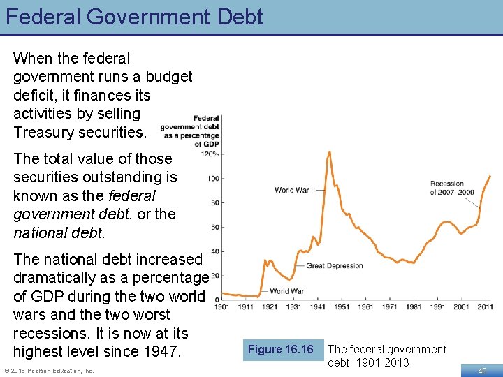
Federal Government Debt When the federal government runs a budget deficit, it finances its activities by selling Treasury securities. The total value of those securities outstanding is known as the federal government debt, or the national debt. The national debt increased dramatically as a percentage of GDP during the two world wars and the two worst recessions. It is now at its highest level since 1947. © 2015 Pearson Education, Inc. Figure 16. 16 The federal government debt, 1901 -2013 48

Is Government Debt a Problem? For now, the federal government is at no serious risk of defaulting on its obligations, because: • The interest rate it can borrow money at is very low • The size of the interest payments on the debt is low relative to the size of the federal budget—around 11% In the long run, a debt that increases in size relative to GDP can pose a problem—potentially crowding out investment, which is a key component of long term growth. • This problem is reduced if the government debt was incurred to finance infrastructure, education, or research and development; these serve as a long term investment for the economy. © 2015 Pearson Education, Inc. 49

The Effects of Fiscal Policy in the Long Run 16. 7 LEARNING OBJECTIVE Discuss

Long-Run Fiscal Policy The fiscal policy we have concentrated on so far was intended to address short-run goals of stabilizing the economy. • But other fiscal policy actions are intended to have long-run impacts on potential GDP—i. e. on aggregate supply, rather than aggregate demand. • Hence these actions are often referred to as supply-side economics. Most such policies are based on changing taxes in order to increase incentives to work, save, invest, and start a business. © 2015 Pearson Education, Inc. 51

The Long-Run Effects of Tax Policy Most taxes are assessed as a percentage of some economic activity, like individual income, corporate income, or capital gains. • When an individual decides how much to work, he bases the decision on how much an hour of work will increase his ability to consume goods and services—the posttax wage. • When a firm decides how many people to employ, it considers how much it has to pay in total for each worker: the pretax wage. The difference between these is an example of a tax wedge: the difference between the pretax and posttax return to an economic activity. • A large tax wedge distorts the incentives of individuals and firms to take part in economic activities, generally resulting in lower levels of economic activity—lower real GDP. © 2015 Pearson Education, Inc. 52

Tax Rates Matter Tax rates matter because the larger they are, the larger will be the behavioral response to the tax: Individual income tax • Affects labor supply decisions and the returns to entrepreneurship Corporate income tax • Affects the incentives of firms to engage in investment Tax on dividends and capital gains • Affects the supply of loanable funds from households to firms, and hence the real interest rate • Also affects the way firms disburse profits— 2003 reduction in dividend tax led some firms like Microsoft to pay dividends for the first time © 2015 Pearson Education, Inc. 53

Tax Simplification Simpler taxes would also lead to economic gains for society. • The current tax code is extremely complicated—over 3, 000 pages long. • The IRS estimates that taxpayers spend more than 6. 4 billion hours each year filling out their tax returns— 45 hours per tax return. • A simplified tax code would increase economic efficiency by reducing the number of decisions households and firms make solely to reduce their tax payments. © 2015 Pearson Education, Inc. 54

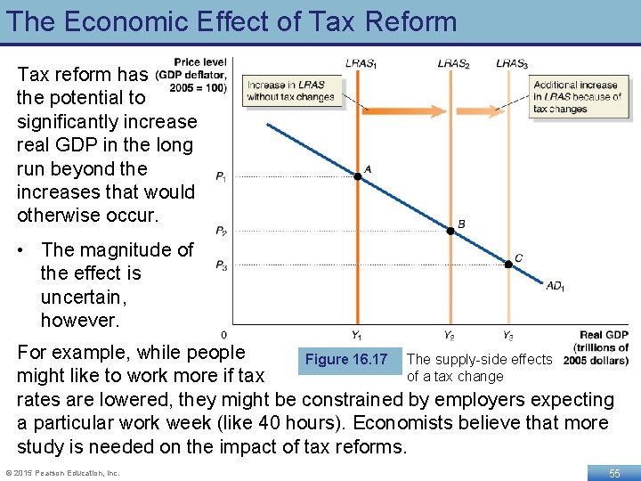
The Economic Effect of Tax Reform Tax reform has the potential to significantly increase real GDP in the long run beyond the increases that would otherwise occur. • The magnitude of the effect is uncertain, however. For example, while people Figure 16. 17 The supply-side effects of a tax change might like to work more if tax rates are lowered, they might be constrained by employers expecting a particular work week (like 40 hours). Economists believe that more study is needed on the impact of tax reforms. © 2015 Pearson Education, Inc. 55

How Large are Supply-Side Effects? While decreasing tax rates would likely result in more economic activity, the magnitude of the effect is debatable. • Workers may not be able to change their work hours very much • Savings and investment may not be affected much by tax rates So the majority of the effect of tax rate cuts may come through aggregate demand. The debate over the magnitude of supply-side effects can only be resolved through careful study. • But even recent work by leading economists has conflicting conclusions. • Hopefully, further study will bring estimates closer together. © 2015 Pearson Education, Inc. 56

Common Misconceptions to Avoid Fiscal policy and monetary policy have similar goals but are different in their methods. Don’t confuse the two. Deficit and debt are not the same. A deficit is the revenue shortfall in a given year, while the debt is the accumulation of prior deficits. A balanced budget is not necessarily good; a budget deficit is not necessarily bad. Government purchases and tax multipliers are for the short run; the long run multipliers are necessarily zero. But just because they are effective only in the short run, does not mean they are unimportant: the short run matters too! © 2015 Pearson Education, Inc. 57

Appendix: A Closer Look at the Multiplier LEARNING OBJECTIVE Apply the multiplier formula. ©

A Closer Look at the Multiplier Our objective in this appendix is to develop an econometric model for how real GDP is determined. Then we will use that model to identify: 1. The government purchases and tax multipliers 2. How those multipliers are altered by tax rates 3. How those multipliers change in an open economy, i. e. when net exports change in response to income changes. Throughout, we will assume that price levels do not change. © 2015 Pearson Education, Inc. 59

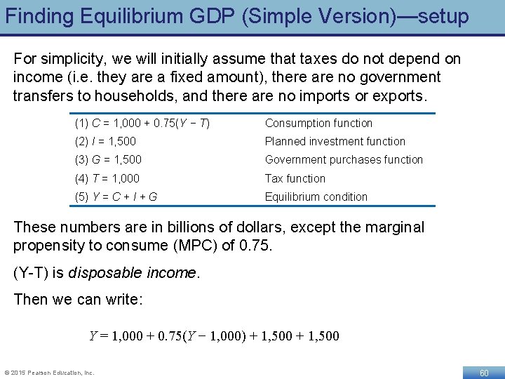
Finding Equilibrium GDP (Simple Version)—setup For simplicity, we will initially assume that taxes do not depend on income (i. e. they are a fixed amount), there are no government transfers to households, and there are no imports or exports. (1) C = 1, 000 + 0. 75(Y − T) Consumption function (2) I = 1, 500 Planned investment function (3) G = 1, 500 Government purchases function (4) T = 1, 000 Tax function (5) Y = C + I + G Equilibrium condition These numbers are in billions of dollars, except the marginal propensity to consume (MPC) of 0. 75. (Y-T) is disposable income. Then we can write: Y = 1, 000 + 0. 75(Y − 1, 000) + 1, 500 © 2015 Pearson Education, Inc. 60

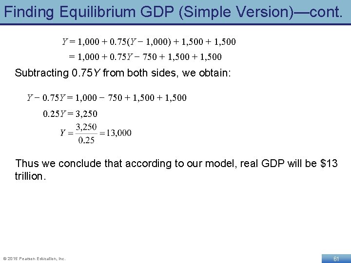
Finding Equilibrium GDP (Simple Version)—cont. Y = 1, 000 + 0. 75(Y − 1, 000) + 1, 500 = 1, 000 + 0. 75 Y − 750 + 1, 500 Subtracting 0. 75 Y from both sides, we obtain: Y − 0. 75 Y = 1, 000 − 750 + 1, 500 0. 25 Y = 3, 250 Thus we conclude that according to our model, real GDP will be $13 trillion. © 2015 Pearson Education, Inc. 61

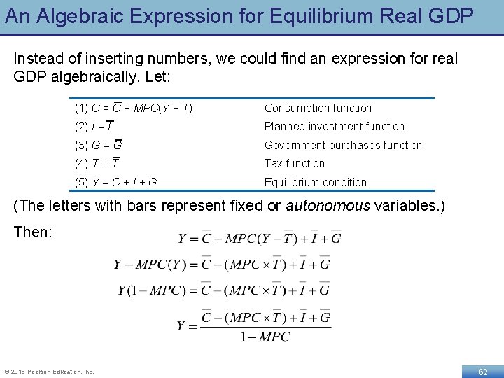
An Algebraic Expression for Equilibrium Real GDP Instead of inserting numbers, we could find an expression for real GDP algebraically. Let: (1) C = C + MPC(Y − T) Consumption function (2) I = I Planned investment function (3) G = G Government purchases function (4) T = T Tax function (5) Y = C + I + G Equilibrium condition (The letters with bars represent fixed or autonomous variables. ) Then: © 2015 Pearson Education, Inc. 62

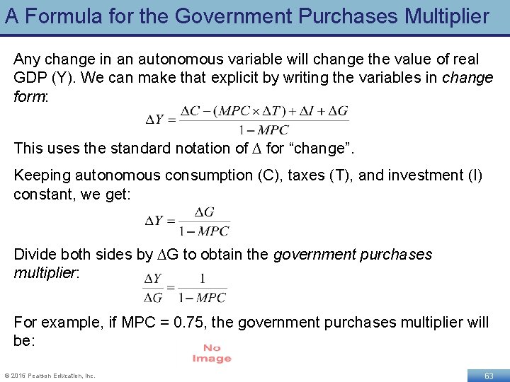
A Formula for the Government Purchases Multiplier Any change in an autonomous variable will change the value of real GDP (Y). We can make that explicit by writing the variables in change form: This uses the standard notation of ∆ for “change”. Keeping autonomous consumption (C), taxes (T), and investment (I) constant, we get: Divide both sides by ∆G to obtain the government purchases multiplier: For example, if MPC = 0. 75, the government purchases multiplier will be: © 2015 Pearson Education, Inc. 63

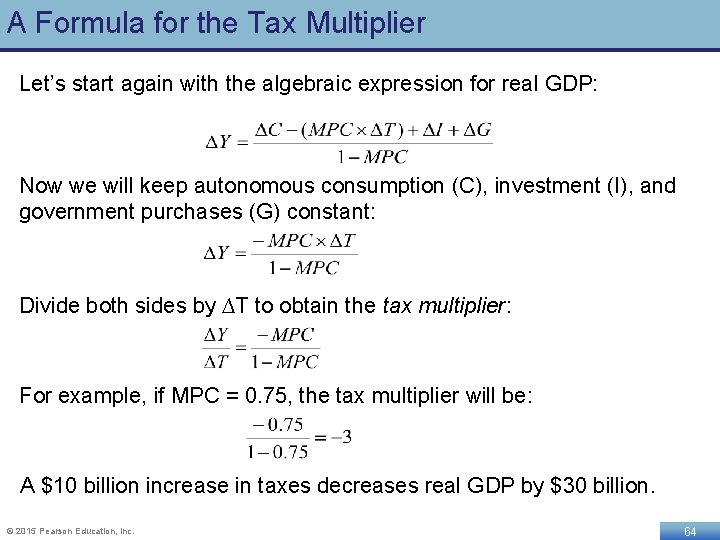
A Formula for the Tax Multiplier Let’s start again with the algebraic expression for real GDP: Now we will keep autonomous consumption (C), investment (I), and government purchases (G) constant: Divide both sides by ∆T to obtain the tax multiplier: For example, if MPC = 0. 75, the tax multiplier will be: A $10 billion increase in taxes decreases real GDP by $30 billion. © 2015 Pearson Education, Inc. 64

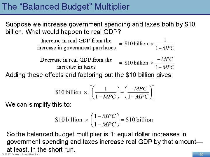
The “Balanced Budget” Multiplier Suppose we increase government spending and taxes both by $10 billion. What would happen to real GDP? Increase in real GDP from the increase in government purchases Decrease in real GDP from the increase in taxes Adding these effects and factoring out the $10 billion gives: We can simplify this to: So the balanced budget multiplier is 1: equal dollar increases in government spending and taxes increase real GDP by that amount— at least, in the short run. © 2015 Pearson Education, Inc. 65

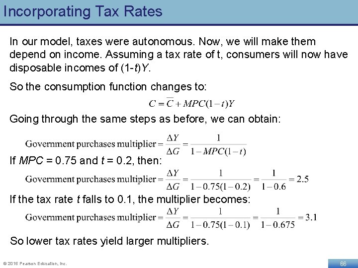
Incorporating Tax Rates In our model, taxes were autonomous. Now, we will make them depend on income. Assuming a tax rate of t, consumers will now have disposable incomes of (1 -t)Y. So the consumption function changes to: Going through the same steps as before, we can obtain: If MPC = 0. 75 and t = 0. 2, then: If the tax rate t falls to 0. 1, the multiplier becomes: So lower tax rates yield larger multipliers. © 2015 Pearson Education, Inc. 66

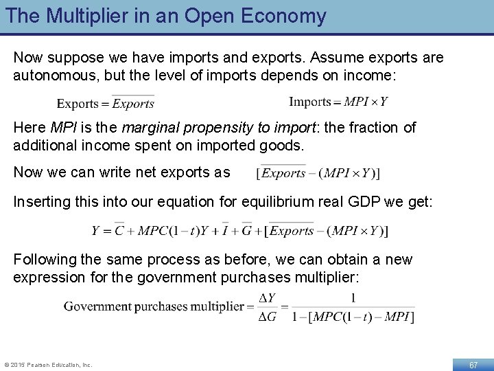
The Multiplier in an Open Economy Now suppose we have imports and exports. Assume exports are autonomous, but the level of imports depends on income: Here MPI is the marginal propensity to import: the fraction of additional income spent on imported goods. Now we can write net exports as Inserting this into our equation for equilibrium real GDP we get: Following the same process as before, we can obtain a new expression for the government purchases multiplier: © 2015 Pearson Education, Inc. 67

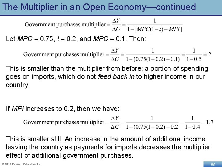
The Multiplier in an Open Economy—continued Let MPC = 0. 75, t = 0. 2, and MPC = 0. 1. Then: This is smaller than the multiplier from before; a portion of spending goes on imports, which do not feed back in to higher income in our country. If MPI increases to 0. 2, then we have: This is smaller still. An increase in the amount of additional income leaving the country as payments for imports decreases the multiplier effect of additional government purchases. © 2015 Pearson Education, Inc. 68