R for Macroecology Spatial data continued Projections Cylindrical

R for Macroecology Spatial data continued

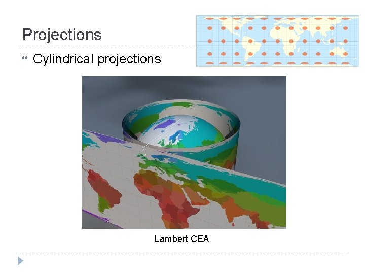
Projections Cylindrical projections Lambert CEA

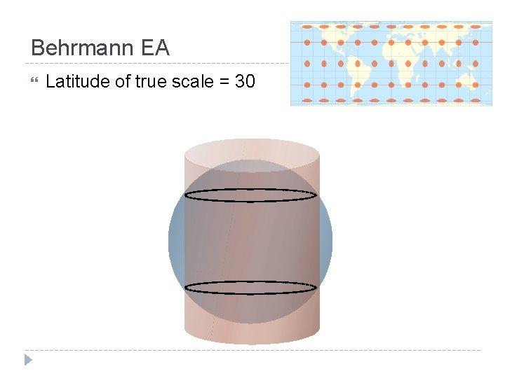
Behrmann EA Latitude of true scale = 30

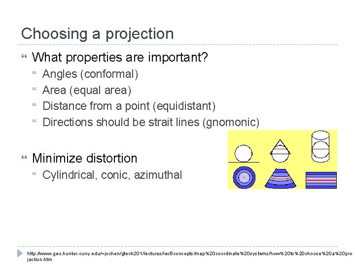
Choosing a projection What properties are important? Angles (conformal) Area (equal area) Distance from a point (equidistant) Directions should be strait lines (gnomonic) Minimize distortion Cylindrical, conic, azimuthal http: //www. geo. hunter. cuny. edu/~jochen/gtech 201/lectures/lec 6 concepts/map%20 coordinate%20 systems/how%20 to%20 choose%20 a%20 pro jection. htm

Projecting points project() function in the proj 4 package is good Can also use project() from rgdal sp. Transform() (in rgdal) works for Spatial. Points, Spatial. Lines, Spatial. Polygons. . . Can also handle transformations from one datum to another

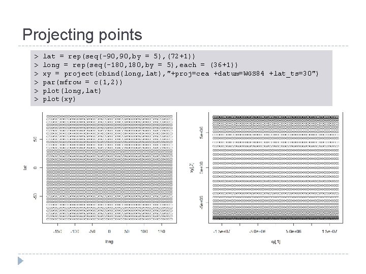
Projecting points > > > lat = rep(seq(-90, by = 5), (72+1)) long = rep(seq(-180, by = 5), each = (36+1)) xy = project(cbind(long, lat), "+proj=cea +datum=WGS 84 +lat_ts=30") par(mfrow = c(1, 2)) plot(long, lat) plot(xy)

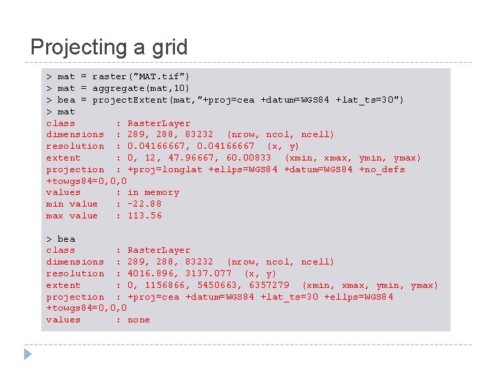
Projecting a grid > mat = raster("MAT. tif") > mat = aggregate(mat, 10) > bea = project. Extent(mat, "+proj=cea +datum=WGS 84 +lat_ts=30") > mat class : Raster. Layer dimensions : 289, 288, 83232 (nrow, ncol, ncell) resolution : 0. 04166667, 0. 04166667 (x, y) extent : 0, 12, 47. 96667, 60. 00833 (xmin, xmax, ymin, ymax) projection : +proj=longlat +ellps=WGS 84 +datum=WGS 84 +no_defs +towgs 84=0, 0, 0 values : in memory min value : -22. 88 max value : 113. 56 > bea class : Raster. Layer dimensions : 289, 288, 83232 (nrow, ncol, ncell) resolution : 4016. 896, 3137. 077 (x, y) extent : 0, 1156866, 5450663, 6357279 (xmin, xmax, ymin, ymax) projection : +proj=cea +datum=WGS 84 +lat_ts=30 +ellps=WGS 84 +towgs 84=0, 0, 0 values : none

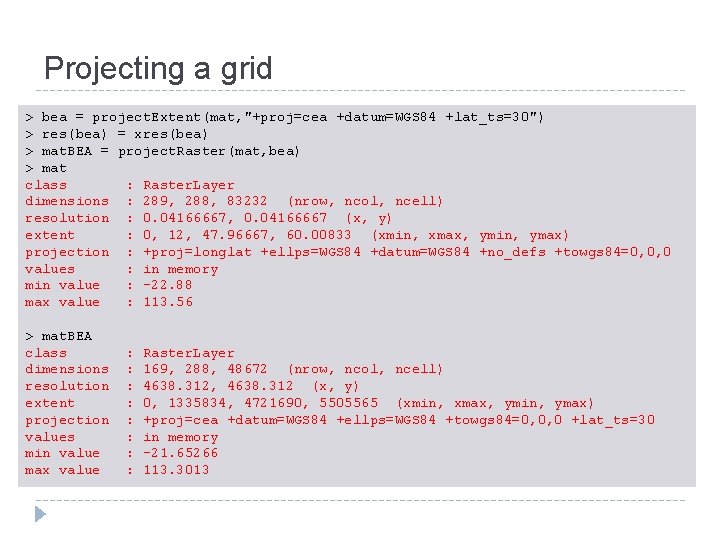
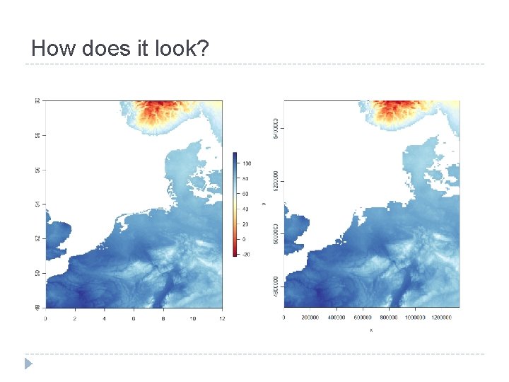
Projecting a grid > bea = project. Extent(mat, "+proj=cea +datum=WGS 84 +lat_ts=30") > res(bea) = xres(bea) > mat. BEA = project. Raster(mat, bea) > mat class : Raster. Layer dimensions : 289, 288, 83232 (nrow, ncol, ncell) resolution : 0. 04166667, 0. 04166667 (x, y) extent : 0, 12, 47. 96667, 60. 00833 (xmin, xmax, ymin, ymax) projection : +proj=longlat +ellps=WGS 84 +datum=WGS 84 +no_defs +towgs 84=0, 0, 0 values : in memory min value : -22. 88 max value : 113. 56 > mat. BEA class dimensions resolution extent projection values min value max value : : : : Raster. Layer 169, 288, 48672 (nrow, ncol, ncell) 4638. 312, 4638. 312 (x, y) 0, 1335834, 4721690, 5505565 (xmin, xmax, ymin, ymax) +proj=cea +datum=WGS 84 +ellps=WGS 84 +towgs 84=0, 0, 0 +lat_ts=30 in memory -21. 65266 113. 3013

How does it look?

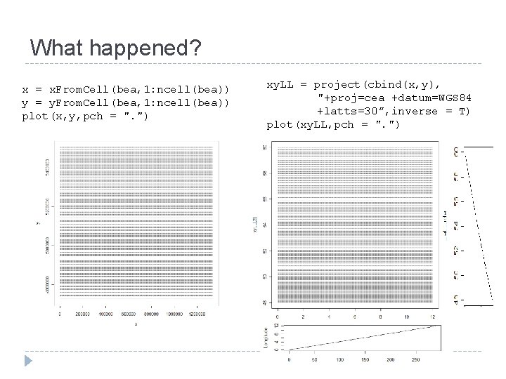
What happened? x = x. From. Cell(bea, 1: ncell(bea)) y = y. From. Cell(bea, 1: ncell(bea)) plot(x, y, pch = ". ") xy. LL = project(cbind(x, y), "+proj=cea +datum=WGS 84 +latts=30”, inverse = T) plot(xy. LL, pch = ". ")

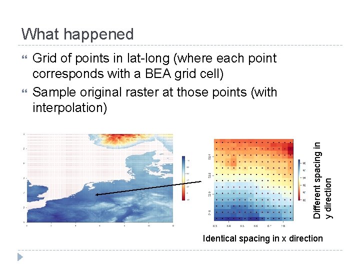
What happened Grid of points in lat-long (where each point corresponds with a BEA grid cell) Sample original raster at those points (with interpolation) Different spacing in y direction Identical spacing in x direction

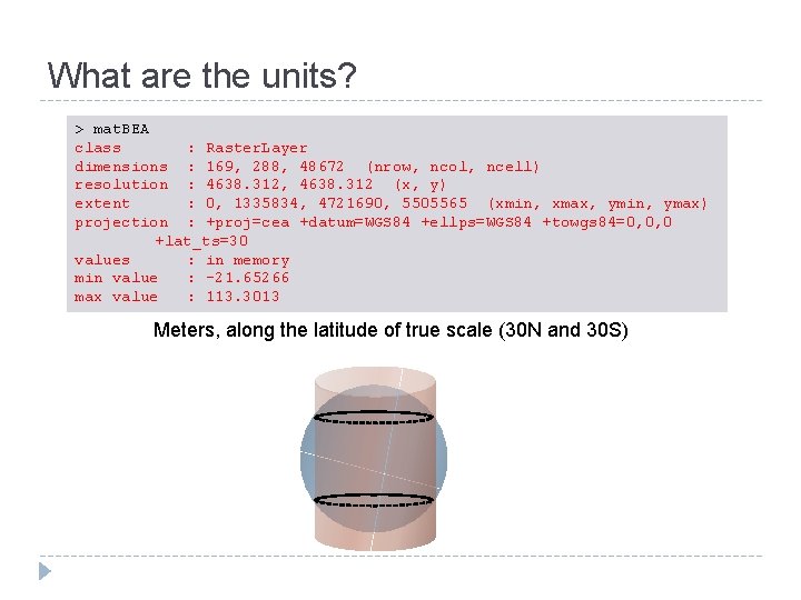
What are the units? > mat. BEA class : Raster. Layer dimensions : 169, 288, 48672 (nrow, ncol, ncell) resolution : 4638. 312, 4638. 312 (x, y) extent : 0, 1335834, 4721690, 5505565 (xmin, xmax, ymin, ymax) projection : +proj=cea +datum=WGS 84 +ellps=WGS 84 +towgs 84=0, 0, 0 +lat_ts=30 values : in memory min value : -21. 65266 max value : 113. 3013 Meters, along the latitude of true scale (30 N and 30 S)

A break to try things out Projections

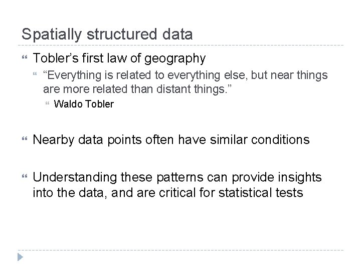
Spatially structured data Tobler’s first law of geography “Everything is related to everything else, but near things are more related than distant things. ” Waldo Tobler Nearby data points often have similar conditions Understanding these patterns can provide insights into the data, and are critical for statistical tests

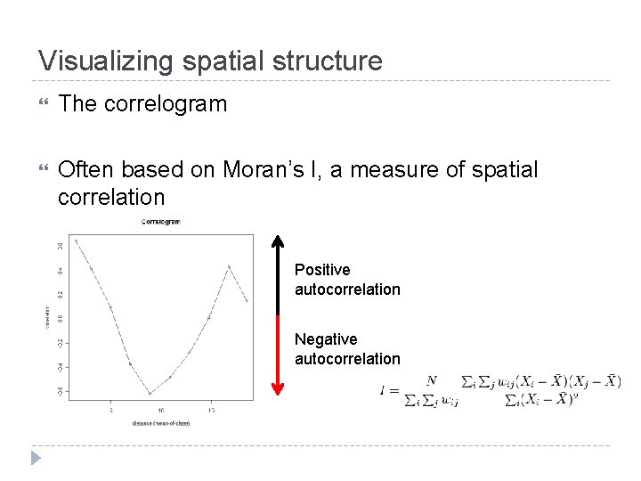
Visualizing spatial structure The correlogram Often based on Moran’s I, a measure of spatial correlation Positive autocorrelation Negative autocorrelation

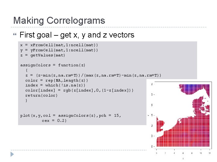
Making Correlograms First goal – get x, y and z vectors x = x. From. Cell(mat, 1: ncell(mat)) y = y. From. Cell(mat, 1: ncell(mat)) z = get. Values(mat) assign. Colors = function(z) { z = (z-min(z, na. rm=T))/(max(z, na. rm=T)-min(z, na. rm=T)) color = rep(NA, length(z)) index = which(!is. na(z)) color[index] = rgb(z[index], 0, (1 -z[index])) return(color) } plot(x, y, col = assign. Colors(z), pch = 15, cex = 0. 2)

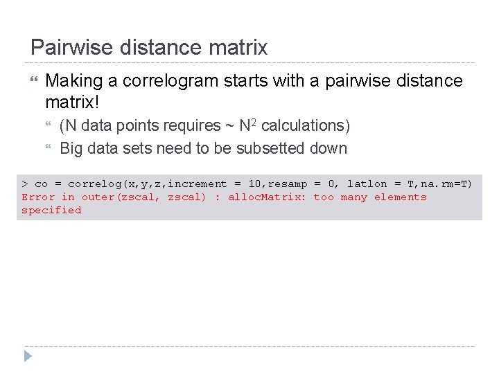
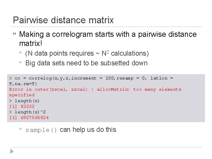
Pairwise distance matrix Making a correlogram starts with a pairwise distance matrix! (N data points requires ~ N 2 calculations) Big data sets need to be subsetted down > co = correlog(x, y, z, increment = 10, resamp = 0, latlon = T, na. rm=T) Error in outer(zscal, zscal) : alloc. Matrix: too many elements specified

Pairwise distance matrix Making a correlogram starts with a pairwise distance matrix! (N data points requires ~ N 2 calculations) Big data sets need to be subsetted down > co = correlog(x, y, z, increment = 100, resamp = 0, latlon = T, na. rm=T) Error in outer(zscal, zscal) : alloc. Matrix: too many elements specified > length(x) [1] 83232 > length(x)^2 [1] 6927565824 sample() can help us do this

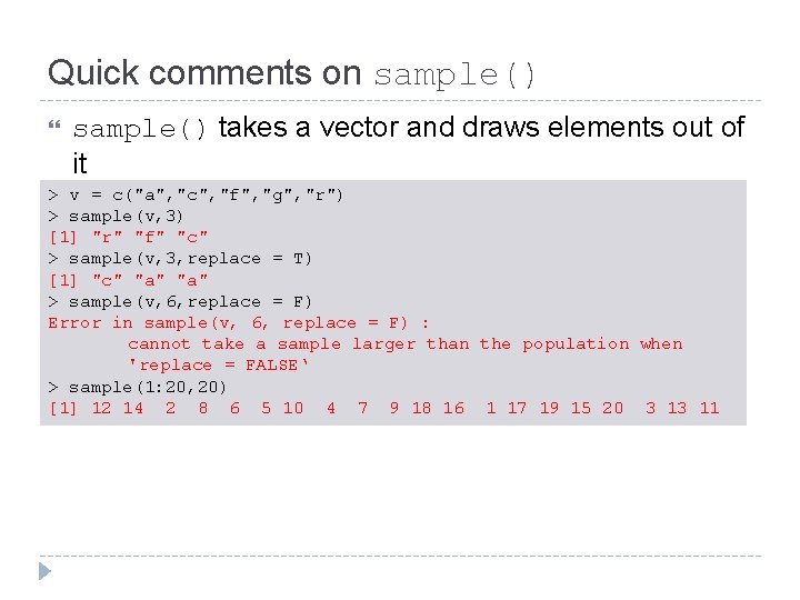
Quick comments on sample() takes a vector and draws elements out of it > v = c("a", "c", "f", "g", "r") > sample(v, 3) [1] "r" "f" "c" > sample(v, 3, replace = T) [1] "c" "a" > sample(v, 6, replace = F) Error in sample(v, 6, replace = F) : cannot take a sample larger than the population when 'replace = FALSE‘ > sample(1: 20, 20) [1] 12 14 2 8 6 5 10 4 7 9 18 16 1 17 19 15 20 3 13 11

Sampling What’s wrong with this? co = correlog( x[sample(1: length(x), 1000, replace = F)], y[sample(1: length(y), 1000, replace = F)], z[sample(1: length(z), 1000, replace = F)], increment = 10, resamp = 0, latlon = T, na. rm=T)

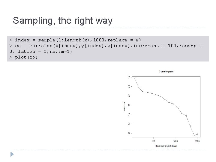
Sampling, the right way > index = sample(1: length(x), 1000, replace = F) > co = correlog(x[index], y[index], z[index], increment = 100, resamp = 0, latlon = T, na. rm=T) > plot(co)

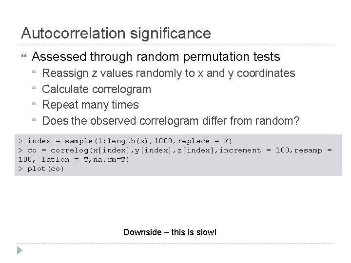
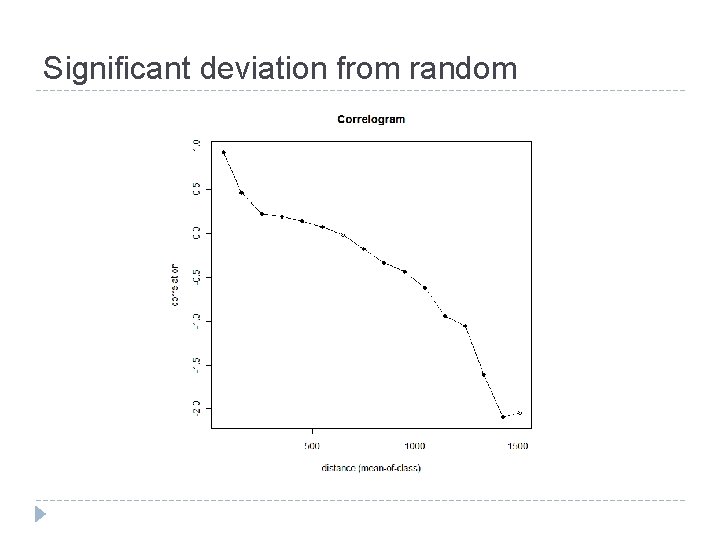
Autocorrelation significance Assessed through random permutation tests Reassign z values randomly to x and y coordinates Calculate correlogram Repeat many times Does the observed correlogram differ from random? > index = sample(1: length(x), 1000, replace = F) > co = correlog(x[index], y[index], z[index], increment = 100, resamp = 100, latlon = T, na. rm=T) > plot(co) Downside – this is slow!

Significant deviation from random

Why is spatial dependence important? Classic statistical tests assume that data points are independent Can bias parameter estimates Leads to incorrect P value estimates A couple of methods to deal with this (next week!) Simultaneous autoregressive models Spatial filters

Just for fun – 3 d surfaces R can render cool 3 d surfaces Demonstrate live rgl. surface() (package rgl)