R E G R a E n a

R E G R a E n a S l y S s i s I O N

SECTION 1 I N T R O D U C T İ O N

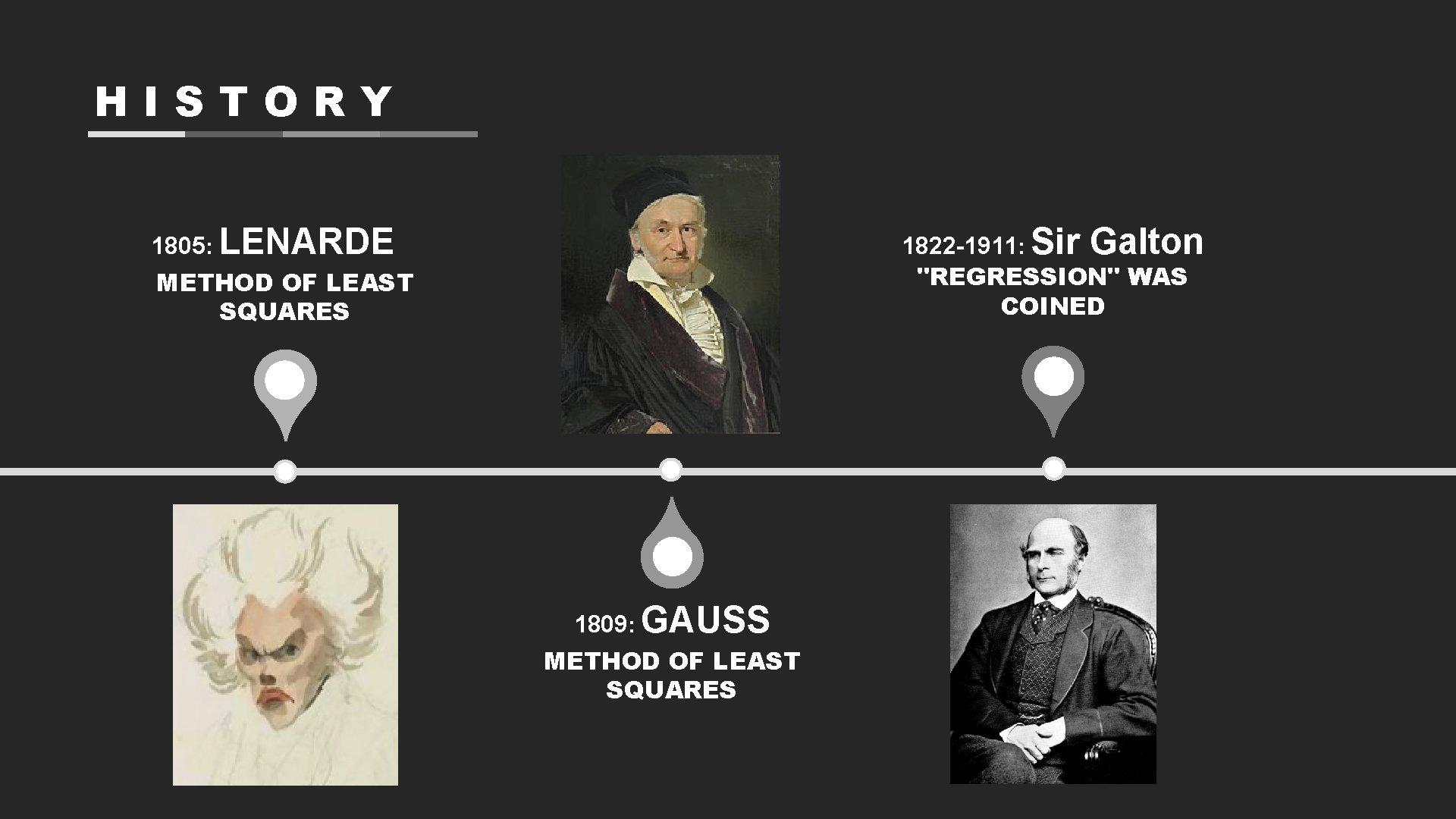
HISTORY 1805: LENARDE 1822 -1911: Sir Galton "REGRESSION" WAS COINED METHOD OF LEAST SQUARES 1809: GAUSS METHOD OF LEAST SQUARES

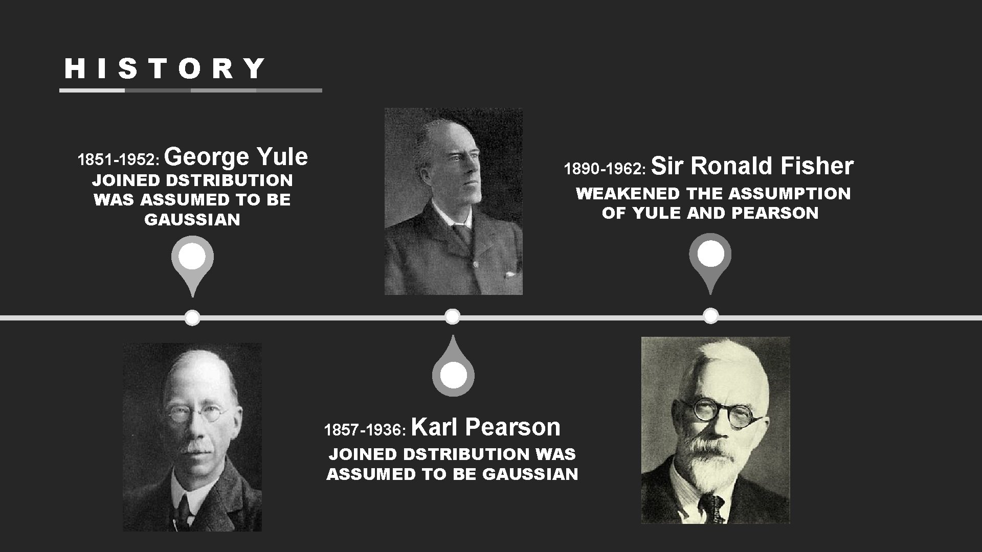
HISTORY 1851 -1952: George Yule JOINED DSTRIBUTION WAS ASSUMED TO BE GAUSSIAN 1890 -1962: Sir Ronald Fisher WEAKENED THE ASSUMPTION OF YULE AND PEARSON 1857 -1936: Karl Pearson JOINED DSTRIBUTION WAS ASSUMED TO BE GAUSSIAN

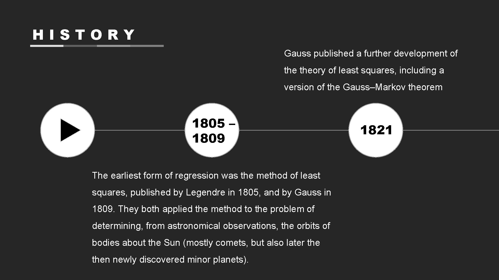
HISTORY Gauss published a further development of theory of least squares, including a version of the Gauss–Markov theorem 1805 – 1809 The earliest form of regression was the method of least squares, published by Legendre in 1805, and by Gauss in 1809. They both applied the method to the problem of determining, from astronomical observations, the orbits of bodies about the Sun (mostly comets, but also later then newly discovered minor planets). 1821

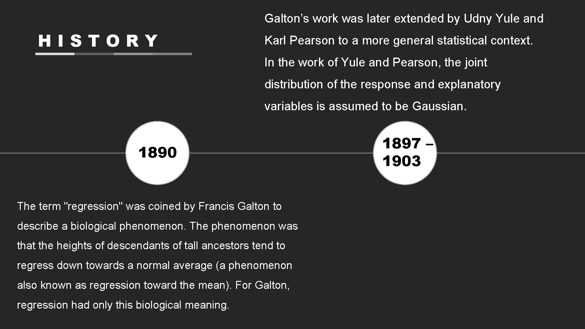
Galton’s work was later extended by Udny Yule and HISTORY Karl Pearson to a more general statistical context. In the work of Yule and Pearson, the joint distribution of the response and explanatory variables is assumed to be Gaussian. 1890 The term "regression" was coined by Francis Galton to describe a biological phenomenon. The phenomenon was that the heights of descendants of tall ancestors tend to regress down towards a normal average (a phenomenon also known as regression toward the mean). For Galton, regression had only this biological meaning. 1897 – 1903

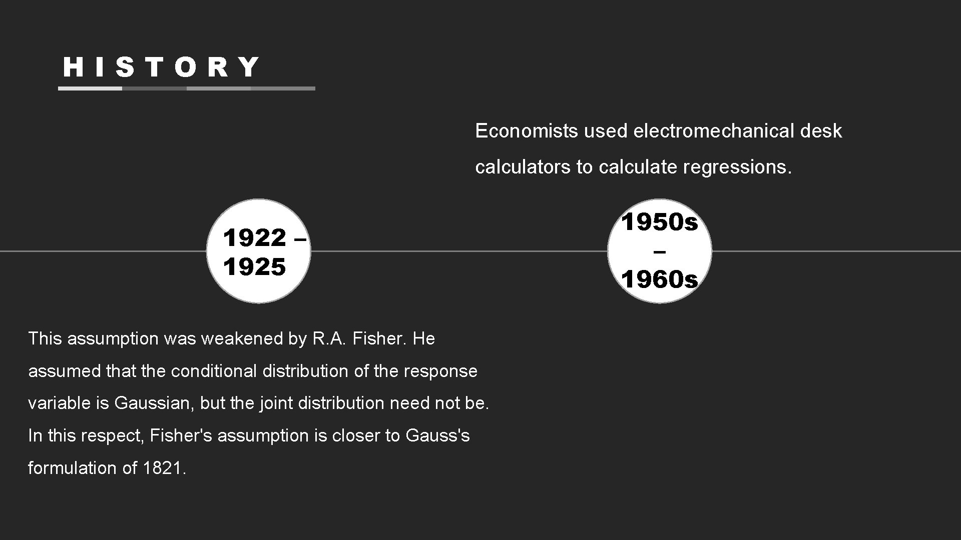
HISTORY Economists used electromechanical desk calculators to calculate regressions. 1922 – 1925 This assumption was weakened by R. A. Fisher. He assumed that the conditional distribution of the response variable is Gaussian, but the joint distribution need not be. In this respect, Fisher's assumption is closer to Gauss's formulation of 1821. 1950 s – 1960 s

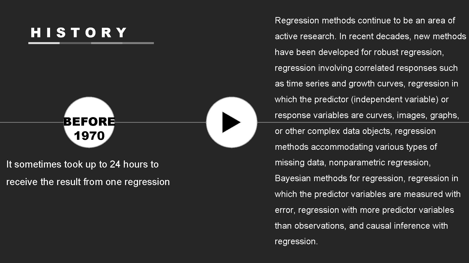
HISTORY Regression methods continue to be an area of active research. In recent decades, new methods have been developed for robust regression, regression involving correlated responses such as time series and growth curves, regression in which the predictor (independent variable) or BEFORE 1970 response variables are curves, images, graphs, or other complex data objects, regression methods accommodating various types of It sometimes took up to 24 hours to missing data, nonparametric regression, receive the result from one regression Bayesian methods for regression, regression in which the predictor variables are measured with error, regression with more predictor variables than observations, and causal inference with regression.

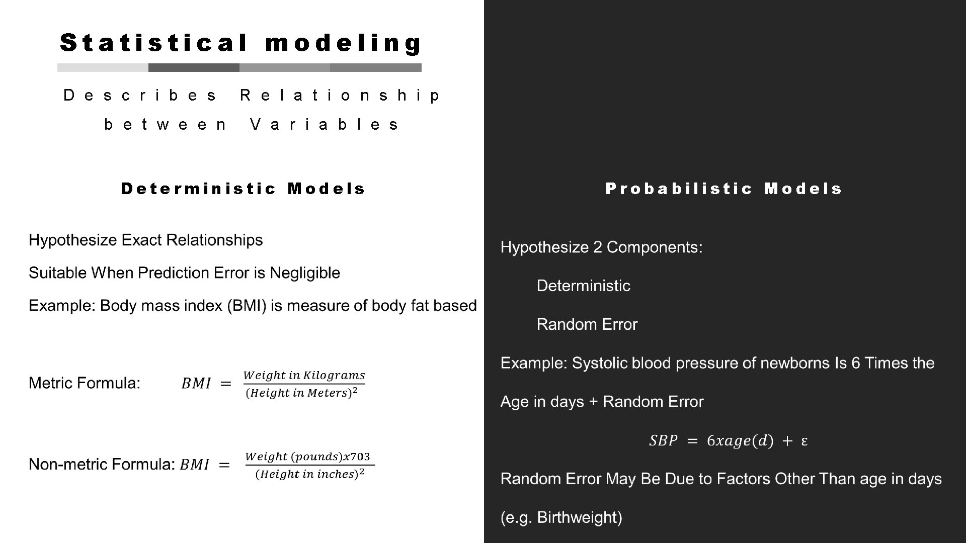
Statistical modeling D e s c r i b e s R e l a t i o n s h i p b e t w e e n V a r i a b l e s Deterministic Models Probabilistic Models

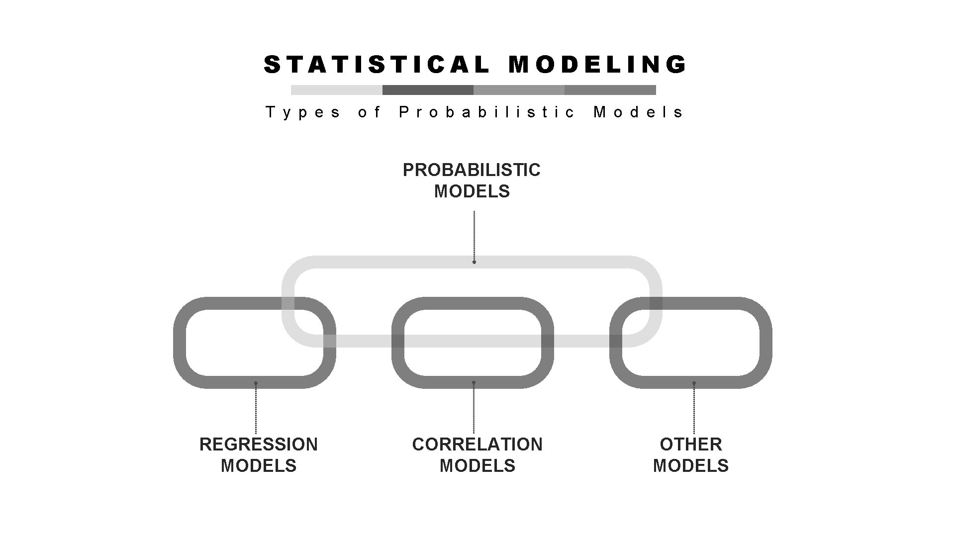
STATISTICAL MODELING T y p e s o f P r o b a b i l i s t i c M o d e l s PROBABILISTIC MODELS REGRESSION MODELS CORRELATION MODELS OTHER MODELS

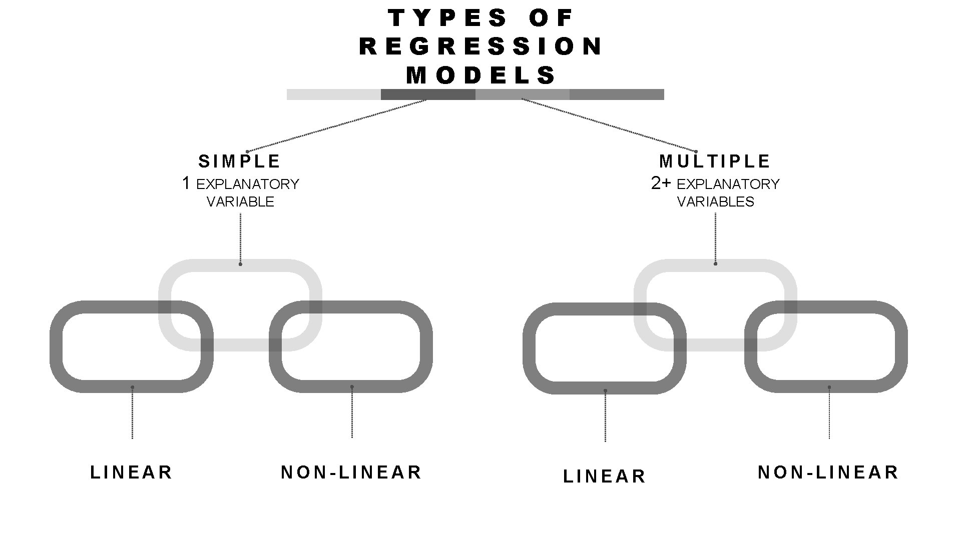
TYPES OF REGRESSION MODELS SIMPLE LINEAR 1 EXPLANATORY MULTIPLE 2+ EXPLANATORY VARIABLES NON-LINEAR NON-LINEAR

REGRESSION a n a l y s i s In analyzing data for the health sciences disciplines, we find that it is frequently desirable to learn something about the relationship between two numeric variables. We may, for example, be interested in studying the relationship between blood pressure and age, height and weight, the concentration of an injected drug and heart rate, the consumption level of some nutrient and weight gain, the intensity of a stimulus and reaction time, or total family income and medical care expenditures. The nature and strength of the relationships between variables such as these may be examined using linear models such as regression and correlation analysis, two statistical techniques that, although related, serve different purposes.

REGRESSION a n a l y s i s Regression analysis is helpful in assessing specific forms of the relationship between variables, and the ultimate objective when this method of analysis is employed usually is to predict or estimate the value of one variable corresponding to a given value of another variable.

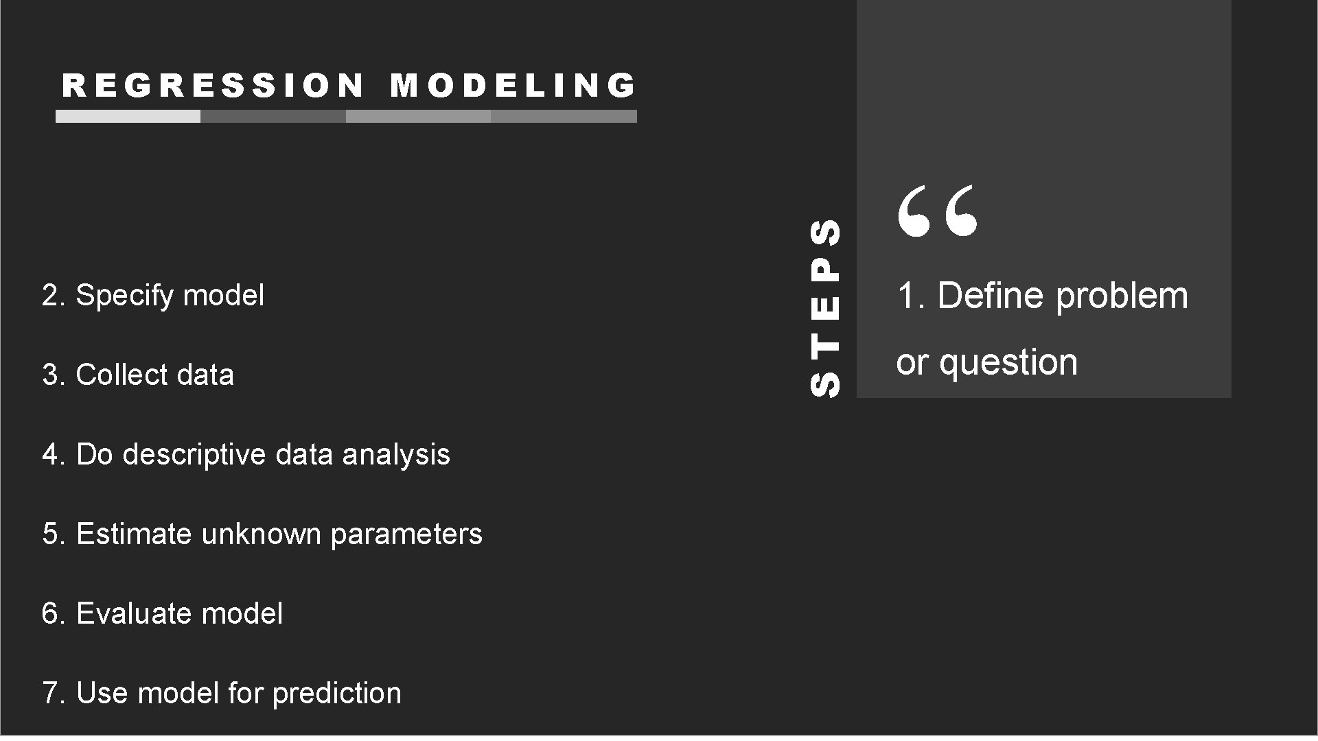
2. Specify model 3. Collect data 4. Do descriptive data analysis 5. Estimate unknown parameters 6. Evaluate model 7. Use model for prediction STEPS REGRESSION MODELING “ 1. Define problem or question

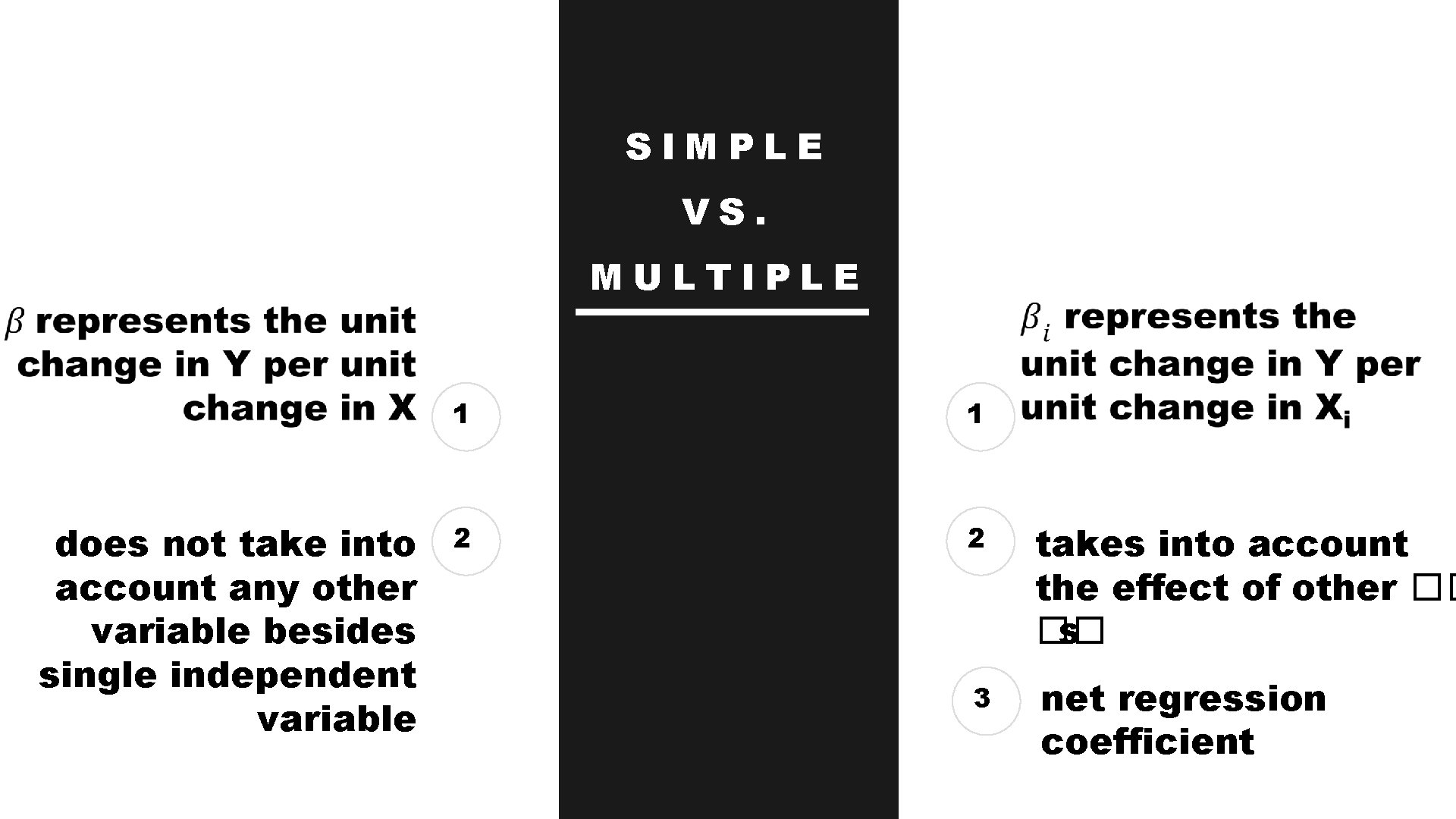
SIMPLE VS. MULTIPLE does not take into account any other variable besides single independent variable 1 1 2 2 takes into account the effect of other �� �� s 3 net regression coefficient

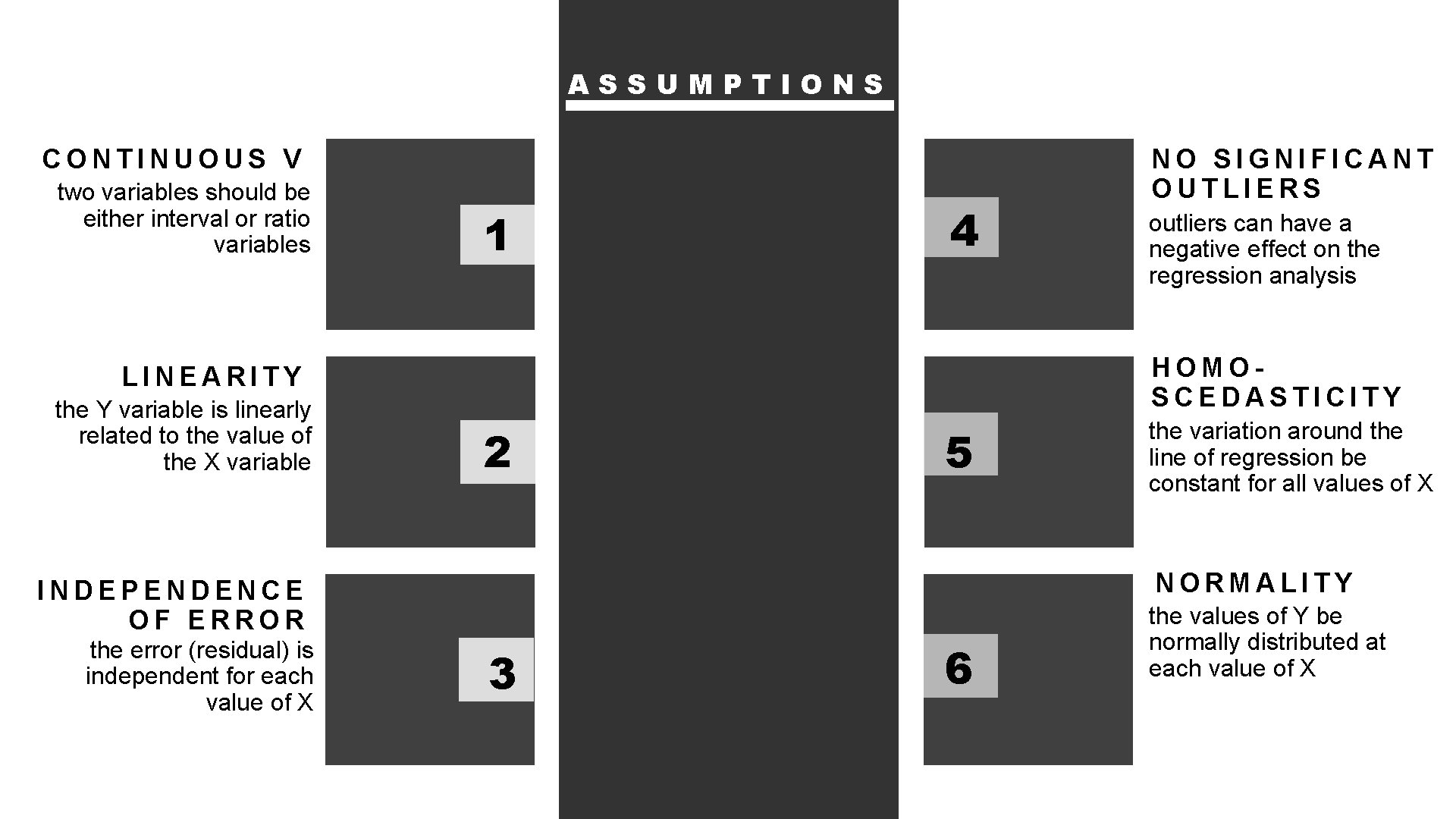
ASSUMPTIONS CONTINUOUS V two variables should be either interval or ratio variables 1 4 2 5 the variation around the line of regression be constant for all values of X NORMALITY INDEPENDENCE OF ERROR the error (residual) is independent for each value of X outliers can have a negative effect on the regression analysis HOMOSCEDASTICITY LINEARITY the Y variable is linearly related to the value of the X variable NO SIGNIFICANT OUTLIERS 3 6 the values of Y be normally distributed at each value of X

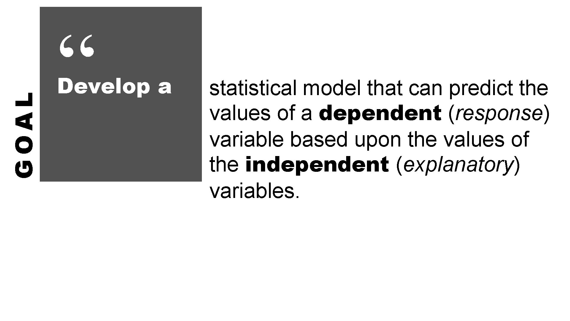
GOAL “ Develop a statistical model that can predict the values of a dependent (response) variable based upon the values of the independent (explanatory) variables.

SECTION 2 L İ N E A R R E G R E S S İ O N A L Y S İ S

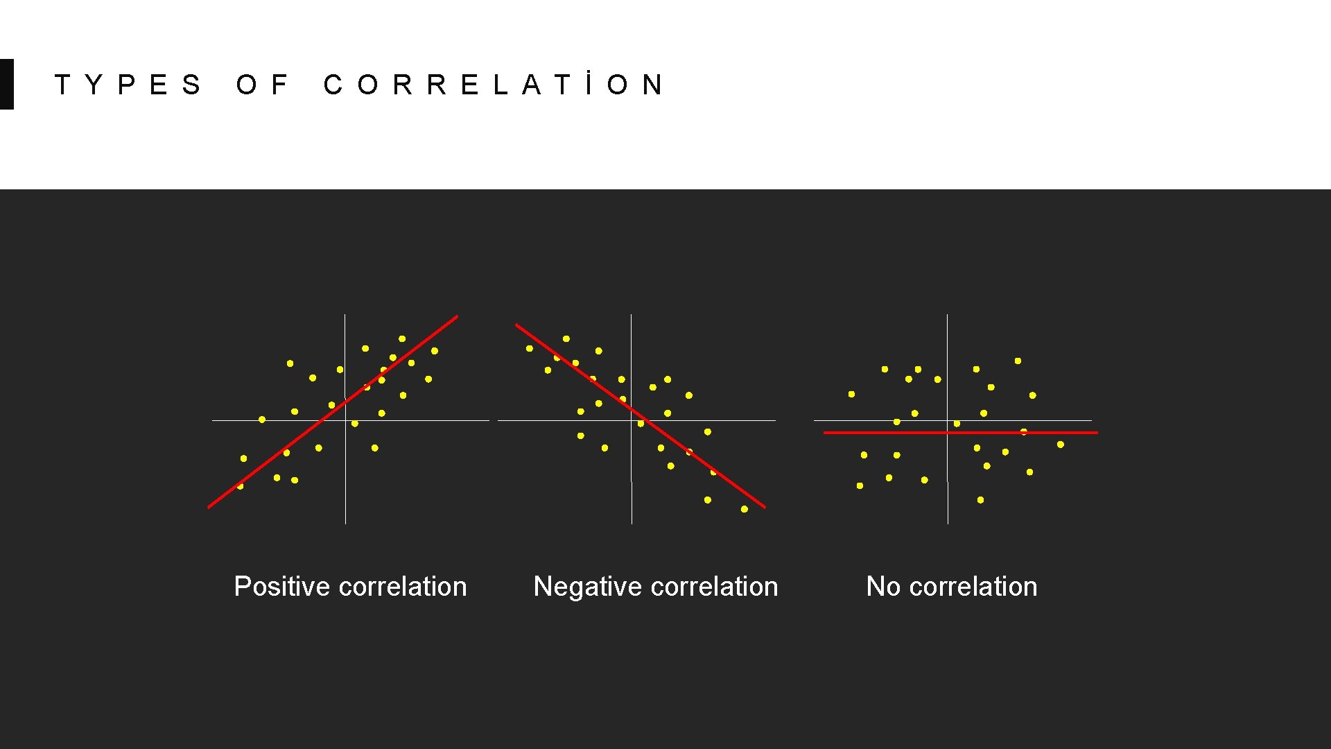
T Y P E S O F C O R R E L A T İ O N Positive correlation Negative correlation No correlation

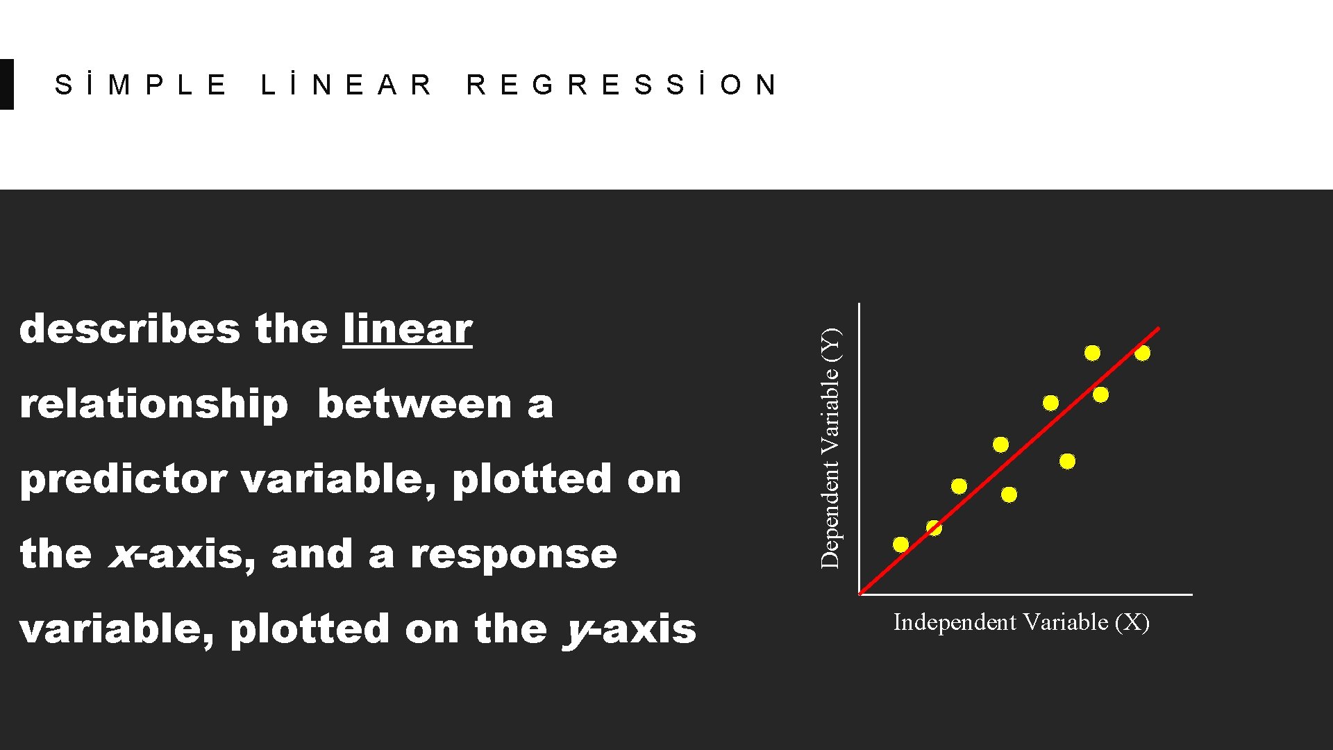
describes the linear relationship between a predictor variable, plotted on the x-axis, and a response variable, plotted on the y-axis Dependent Variable (Y) S İ M P L E L İ N E A R R E G R E S S İ O N Independent Variable (X)

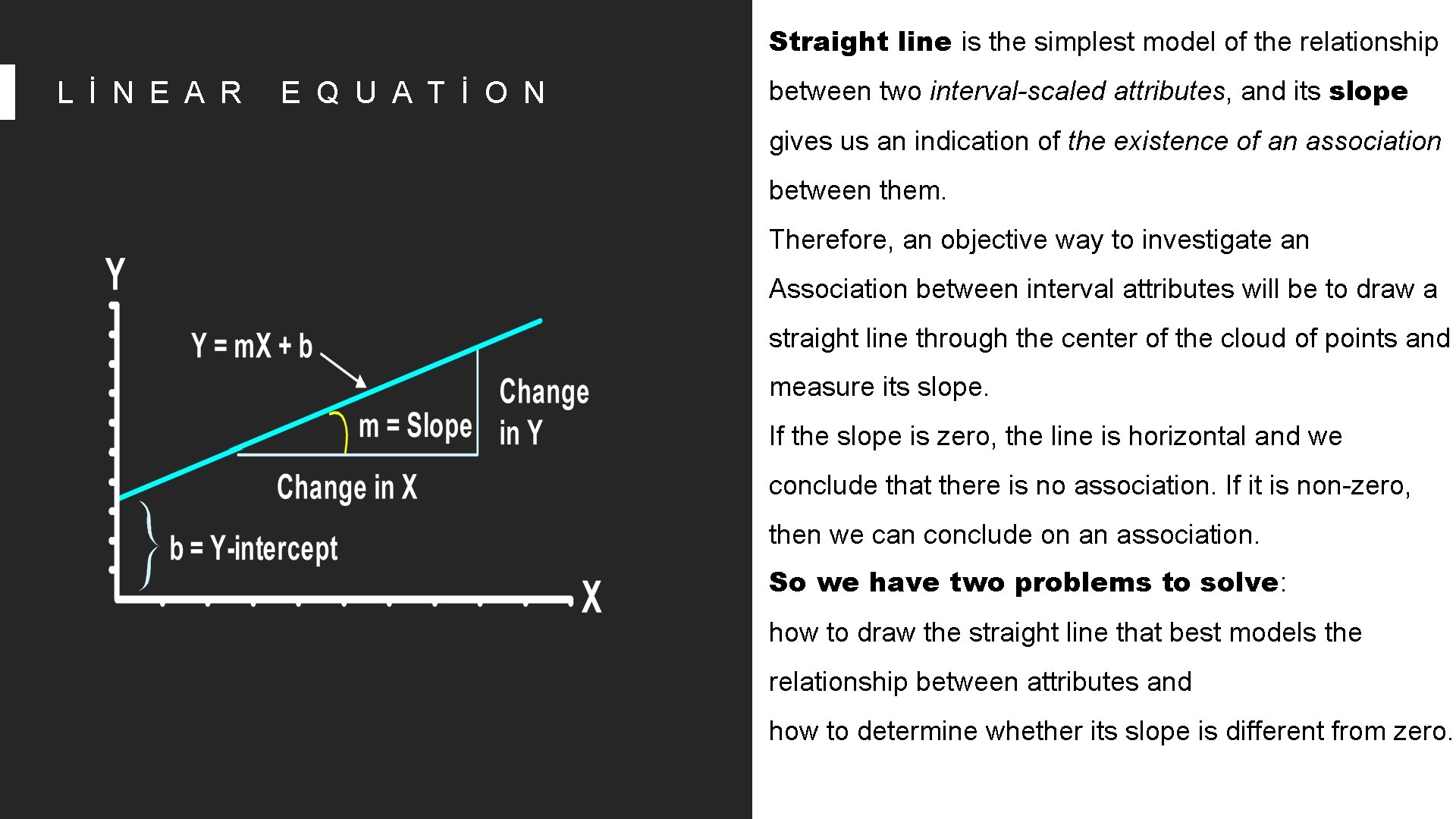
Straight line is the simplest model of the relationship L İ N E A R E Q U A T İ O N between two interval-scaled attributes, and its slope gives us an indication of the existence of an association between them. Therefore, an objective way to investigate an Association between interval attributes will be to draw a straight line through the center of the cloud of points and measure its slope. If the slope is zero, the line is horizontal and we conclude that there is no association. If it is non-zero, then we can conclude on an association. So we have two problems to solve: how to draw the straight line that best models the relationship between attributes and how to determine whether its slope is different from zero.

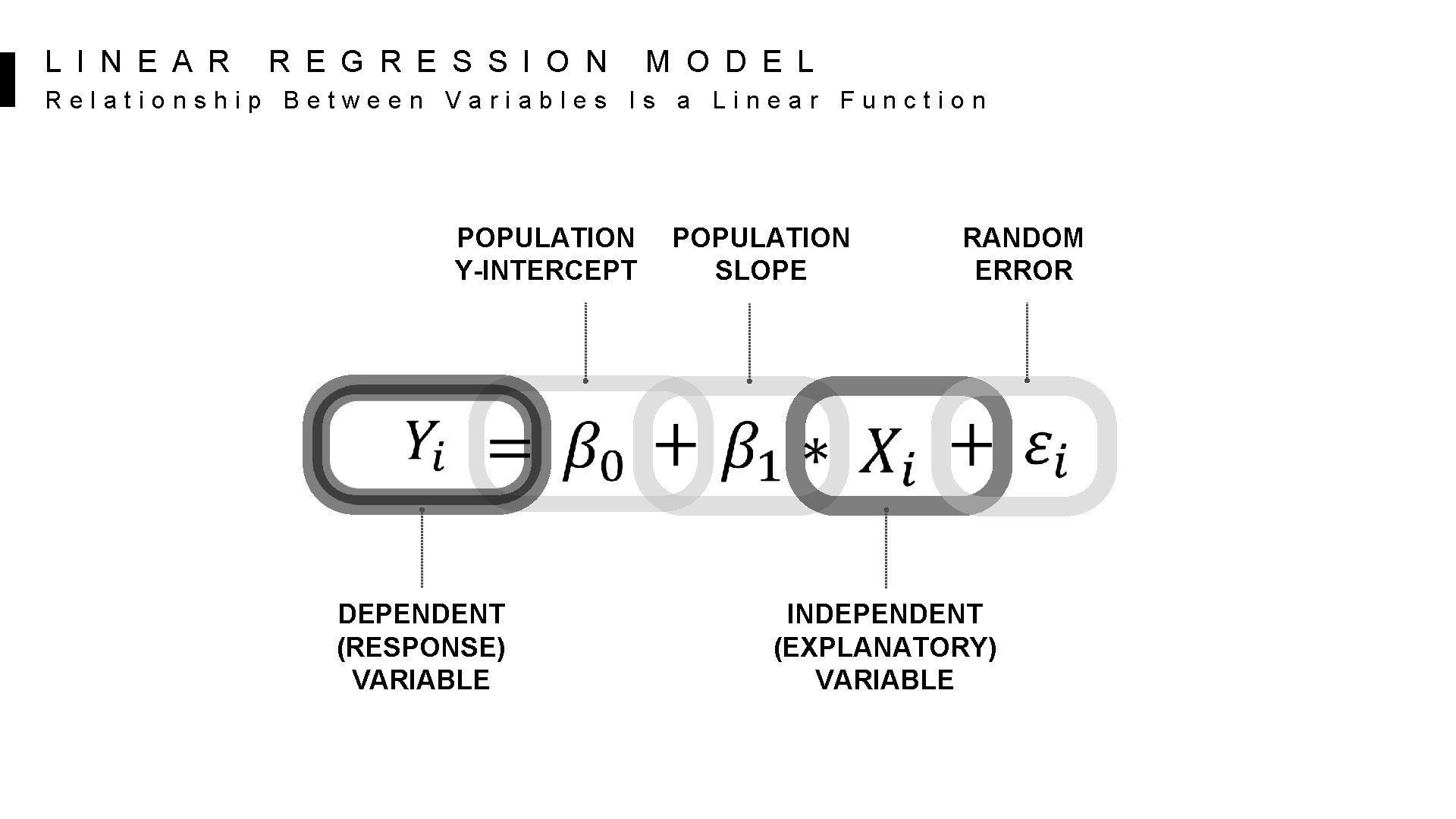
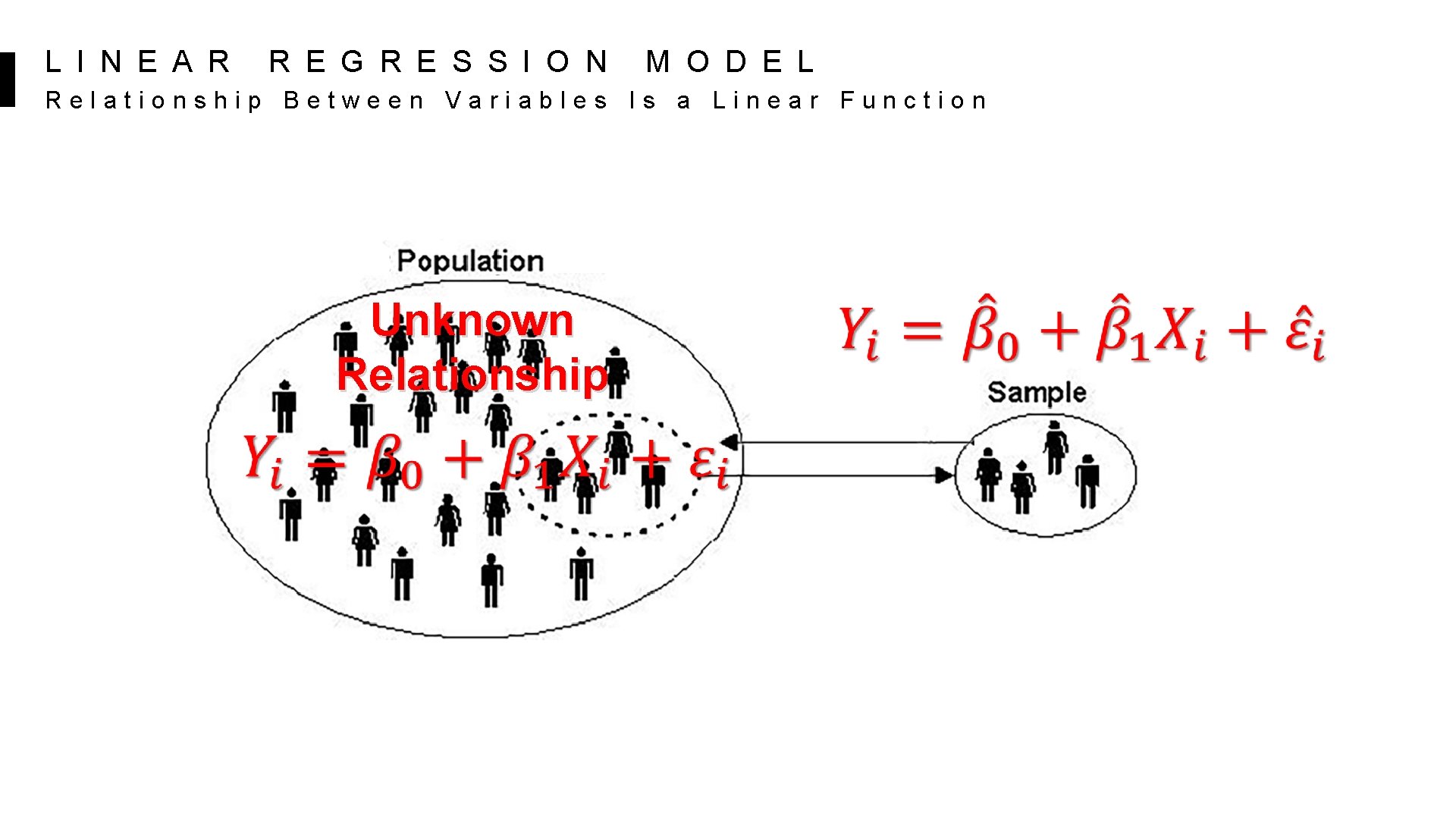
L I N E A R R E G R E S S I O N M O D E L Relationship Between Variables Is a Linear Function POPULATION Y-INTERCEPT DEPENDENT (RESPONSE) VARIABLE POPULATION SLOPE RANDOM ERROR INDEPENDENT (EXPLANATORY) VARIABLE

L I N E A R R E G R E S S I O N M O D E L Relationship Between Variables Is a Linear Function Unknown Relationship

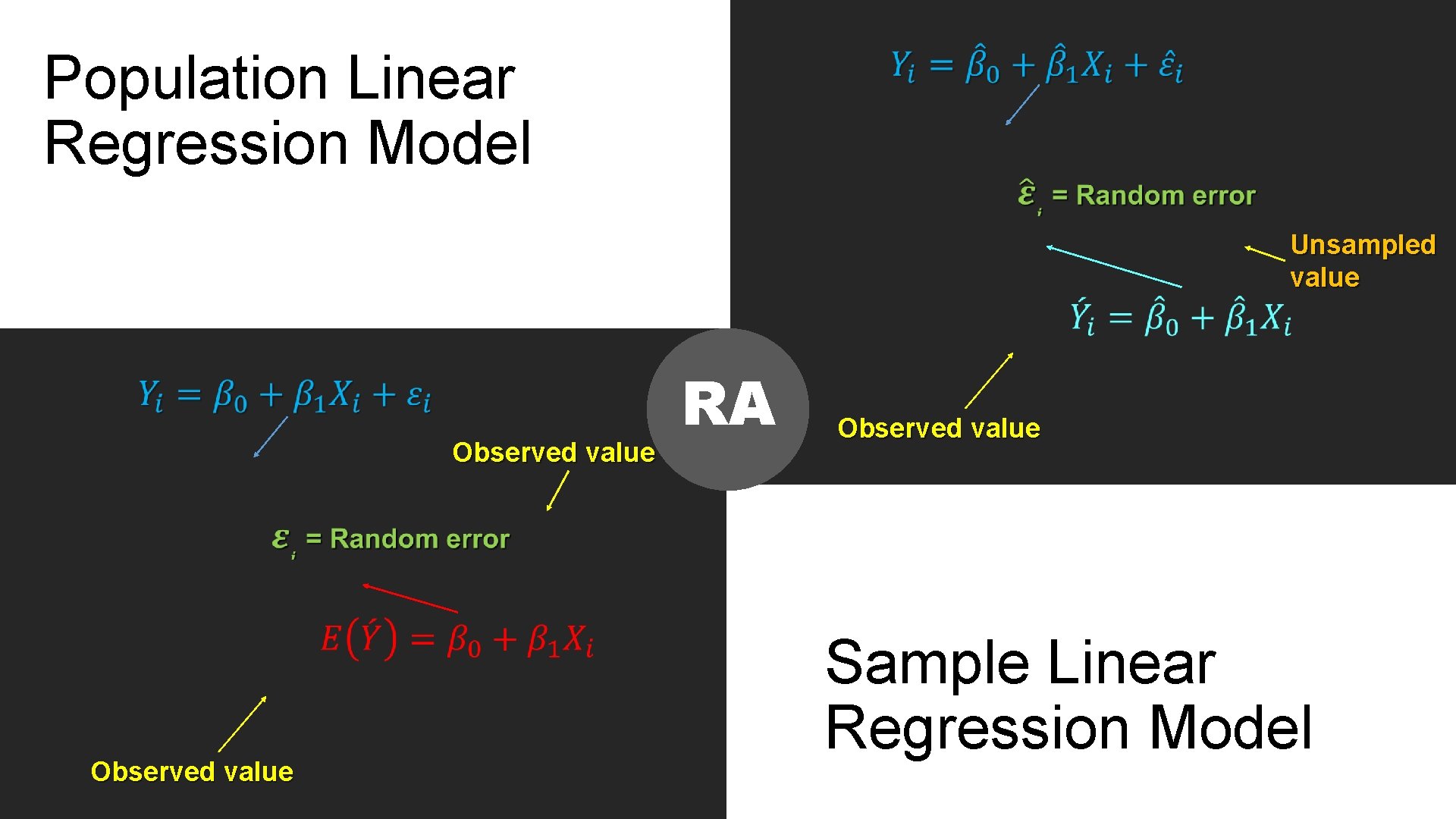
Population Linear Regression Model Unsampled value Observed value RA Observed value Sample Linear Regression Model

SECTION 3 T H E O R D I N A R Y L E A S T S Q U A R E M E T H O D ( O L S )

! THE ORDINARY HOW TO FIT DATA TO LEAST SQUARE A LINEAR MODEL? METHOD (OLS)

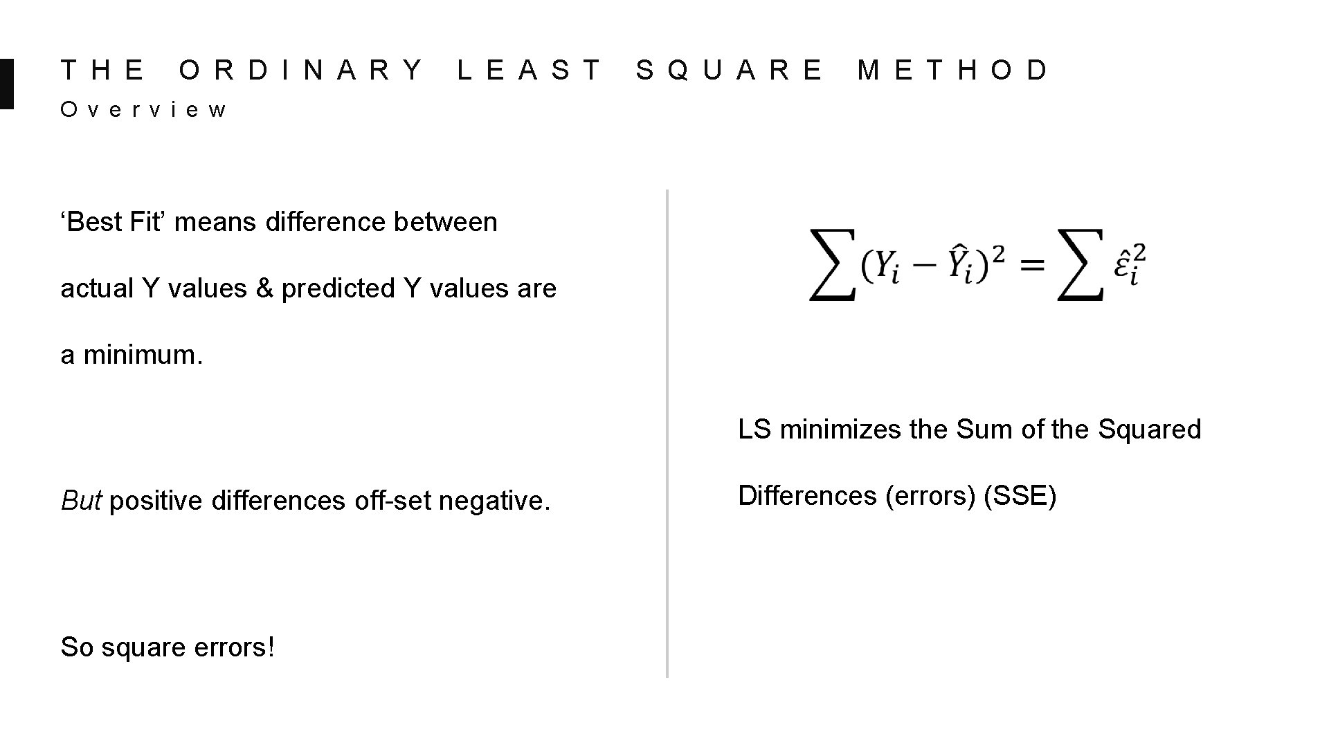
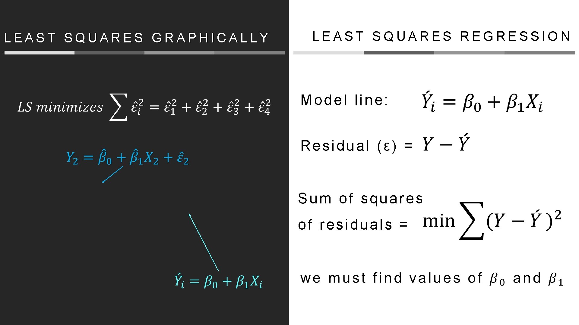
T H E O R D I N A R Y L E A S T S Q U A R E M E T H O D O v e r v i e w ‘Best Fit’ means difference between actual Y values & predicted Y values are a minimum. LS minimizes the Sum of the Squared But positive differences off-set negative. So square errors! Differences (errors) (SSE)

LEAST SQUARES REGRESSION LEAST SQUARES GRAPHICALLY Model line: Residual (ε) = S u m o f s q u a r e s of residuals =

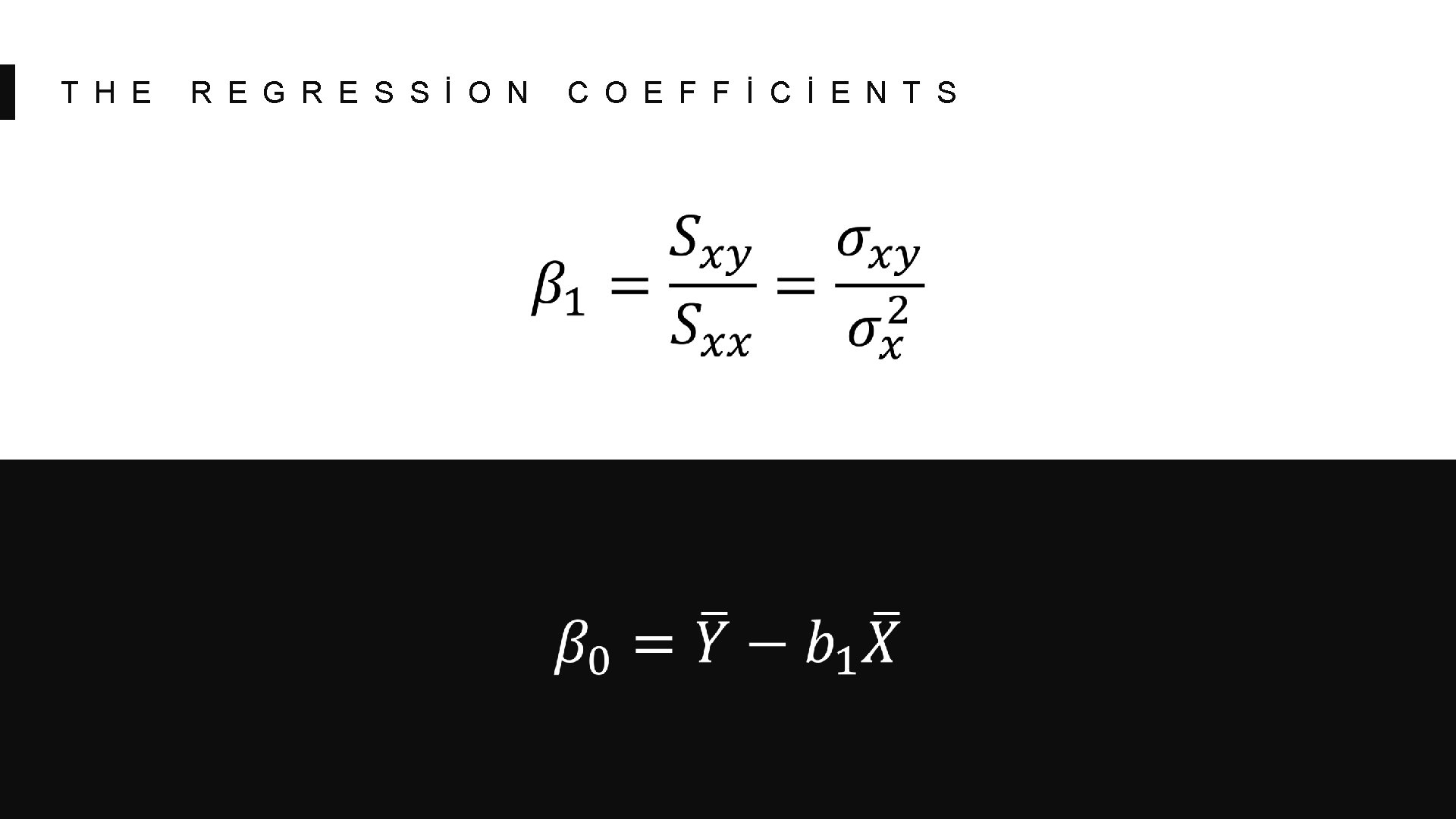
T H E R E G R E S S İ O N C O E F F İ C İ E N T S

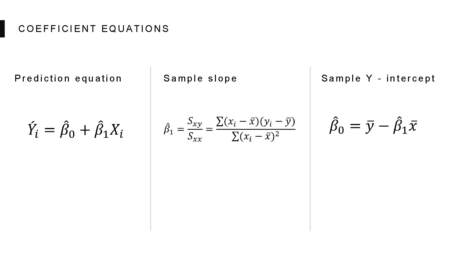
COEFFICIENT EQUATIONS Prediction equation Sample slope Sample Y - intercept

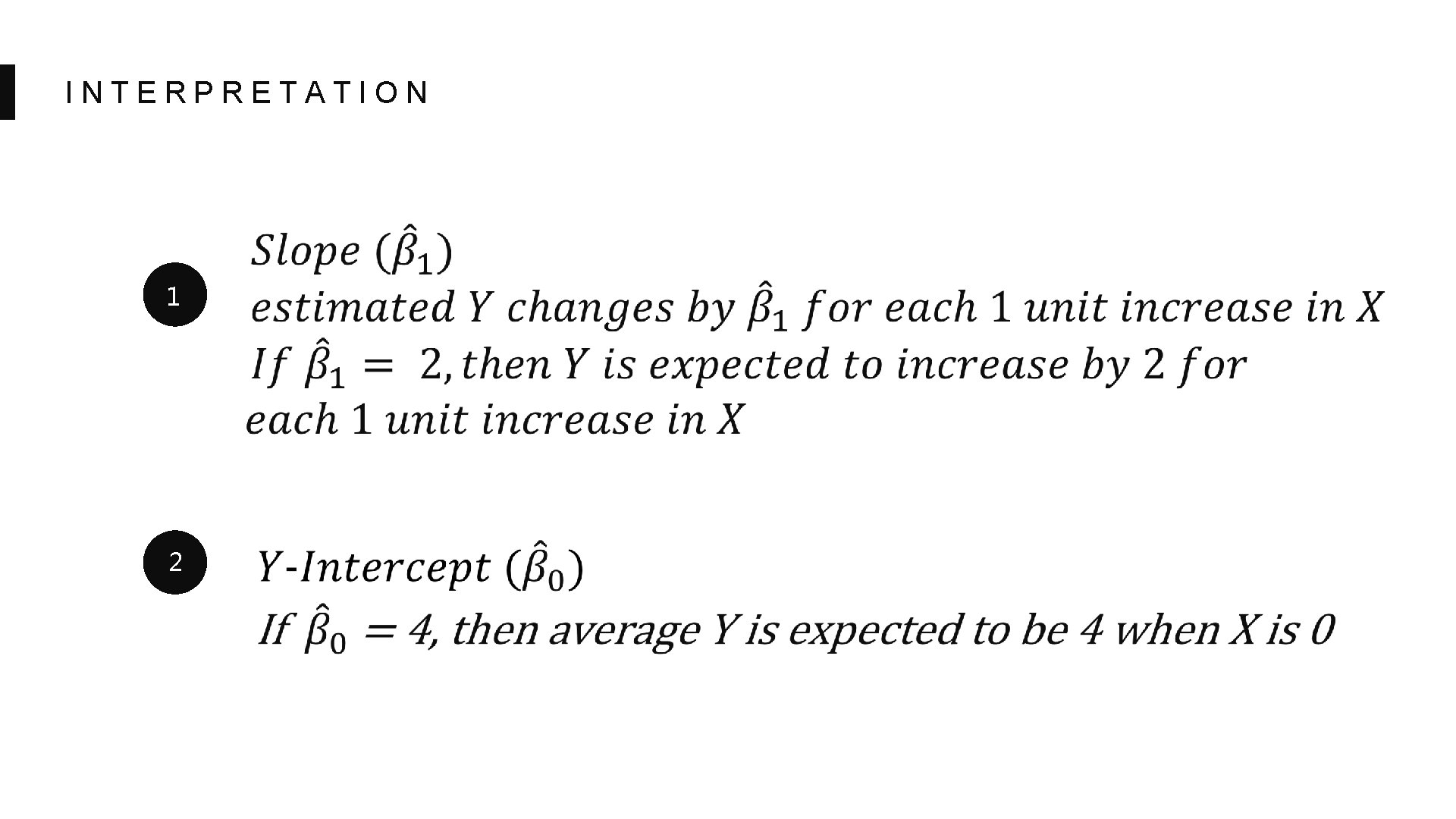
INTERPRETATION 1 2

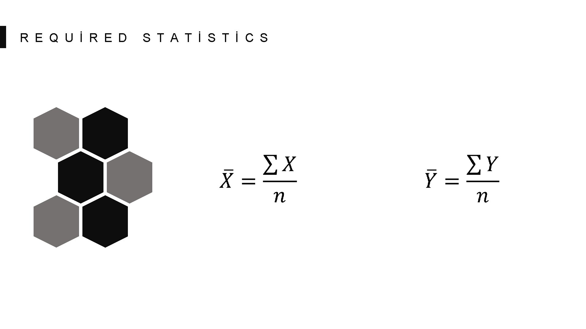
R E Q U İ R E D S T A T İ S T İ C S

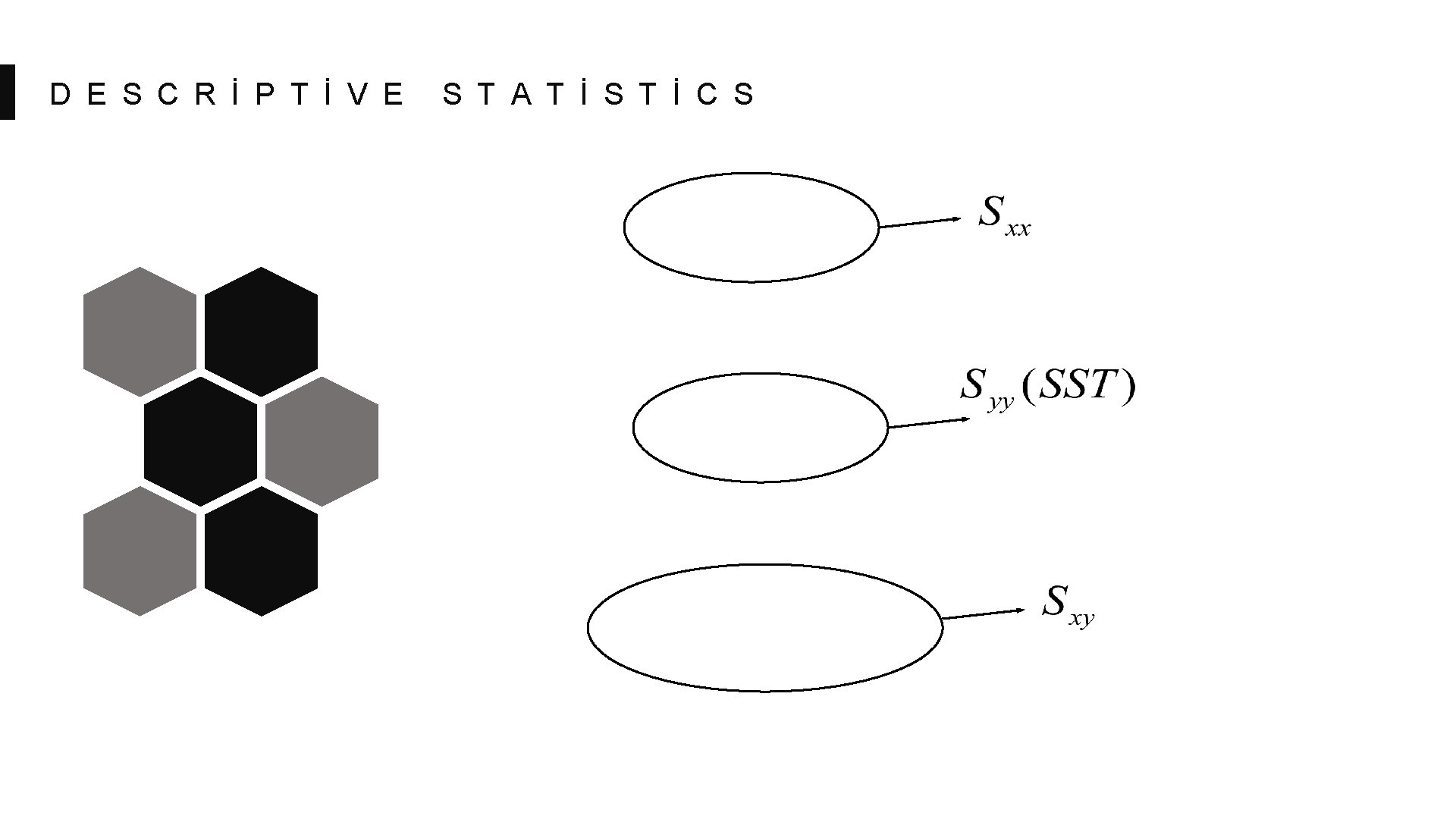
D E S C R İ P T İ V E S T A T İ S T İ C S

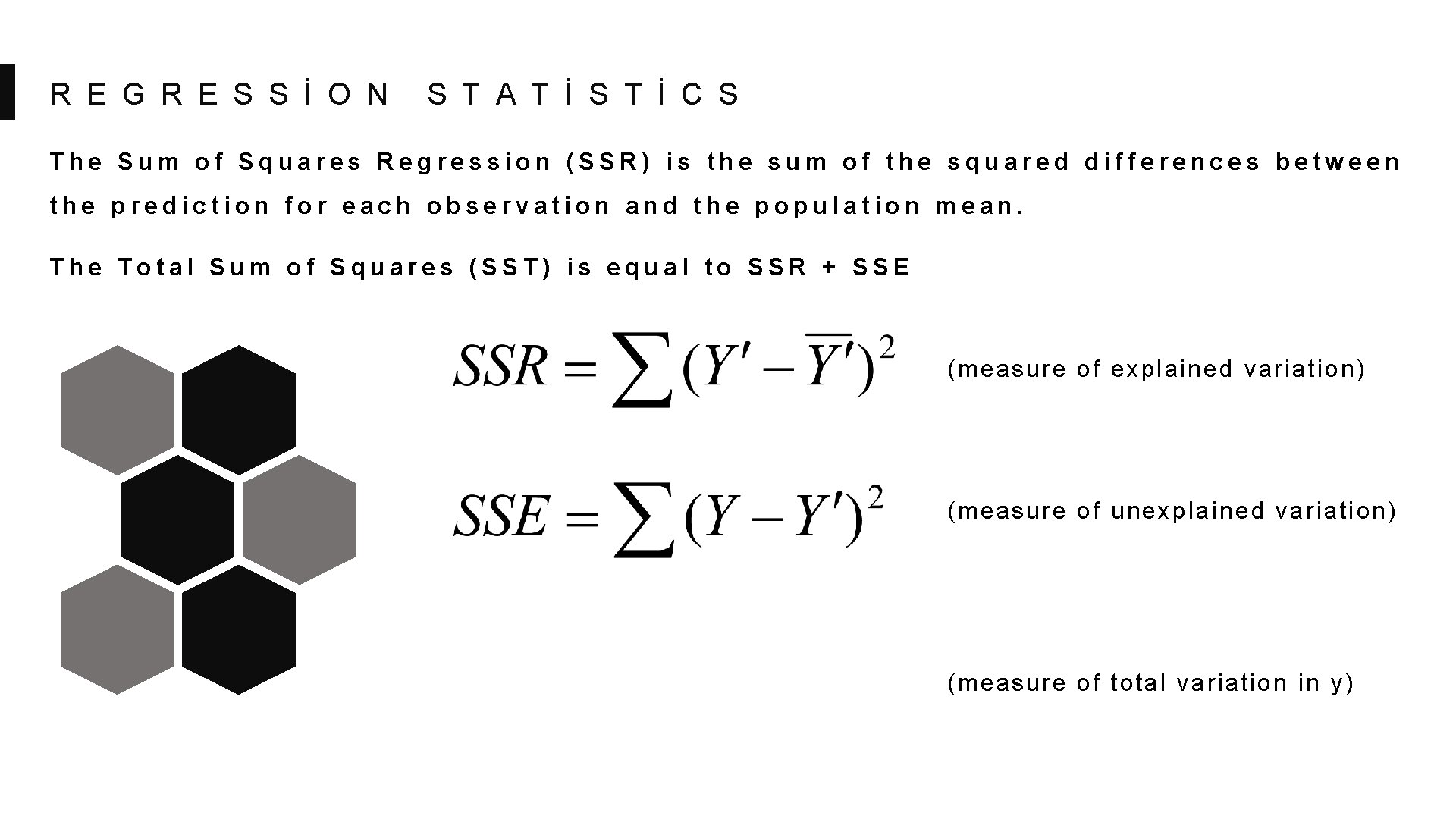
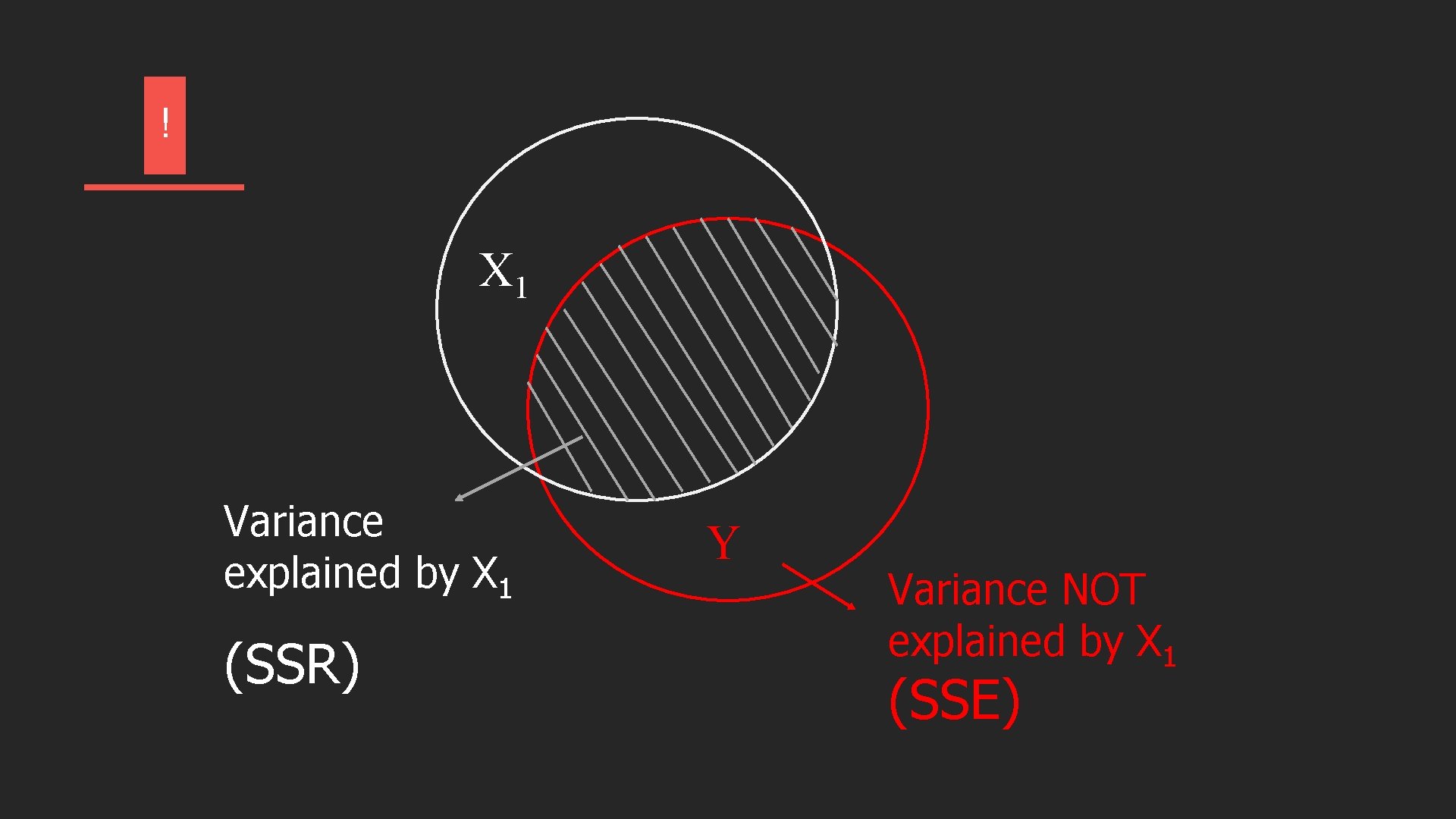
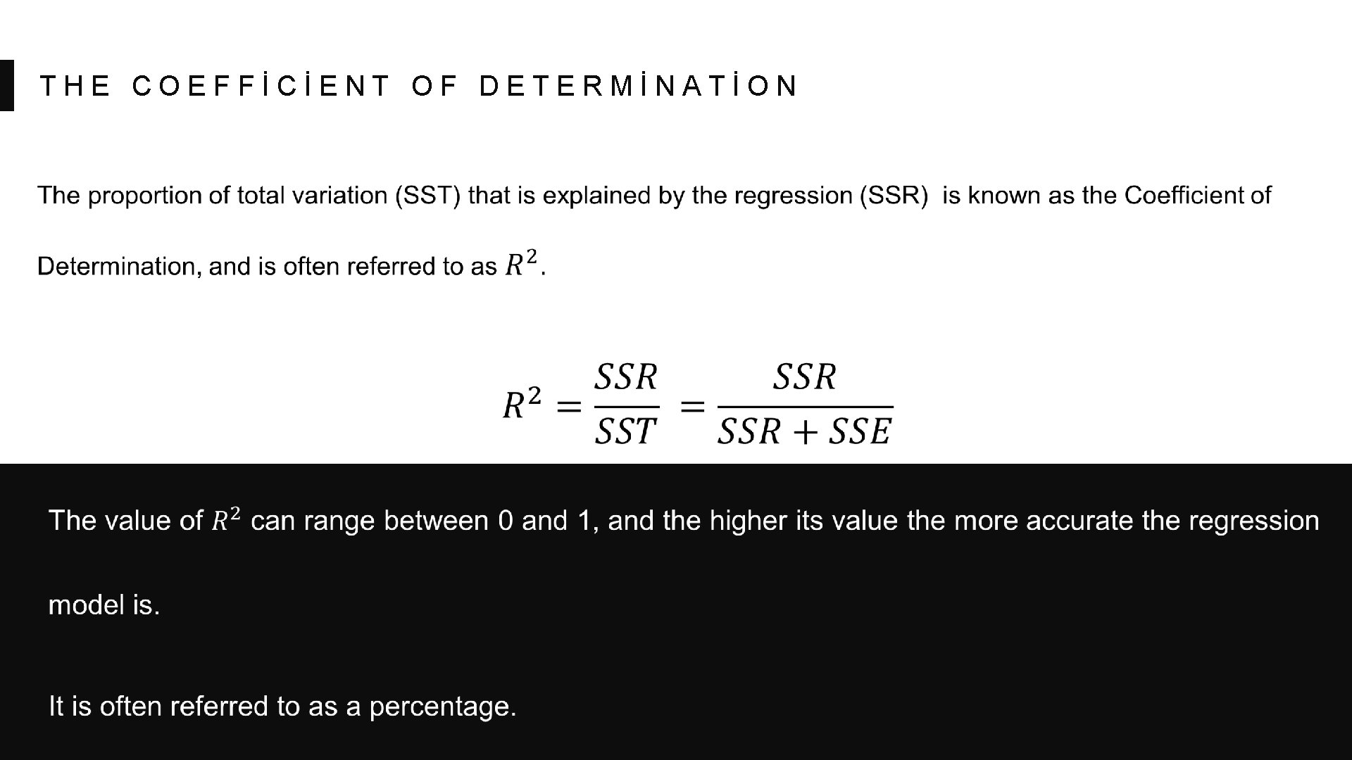
R E G R E S S İ O N S T A T İ S T İ C S The Sum of Squares Regression (SSR) is the sum of the squared differences between the prediction for each observation and the population mean. The Total Sum of Squares (SST) is equal to SSR + SSE (measure of explained variation) (measure of unexplained variation) (measure of total variation in y)

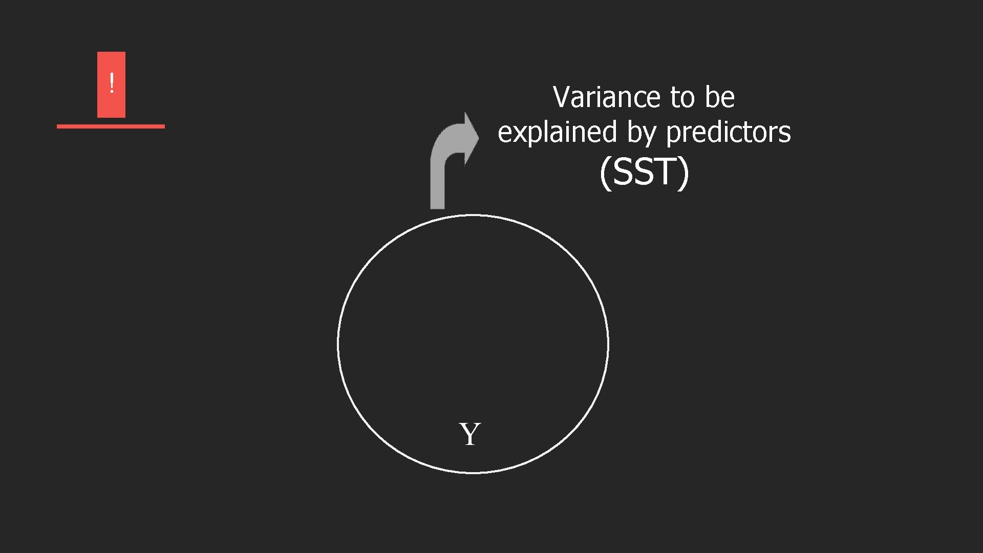
! Variance to be explained by predictors (SST) Y

! X 1 Variance explained by X 1 (SSR) Y Variance NOT explained by X 1 (SSE)

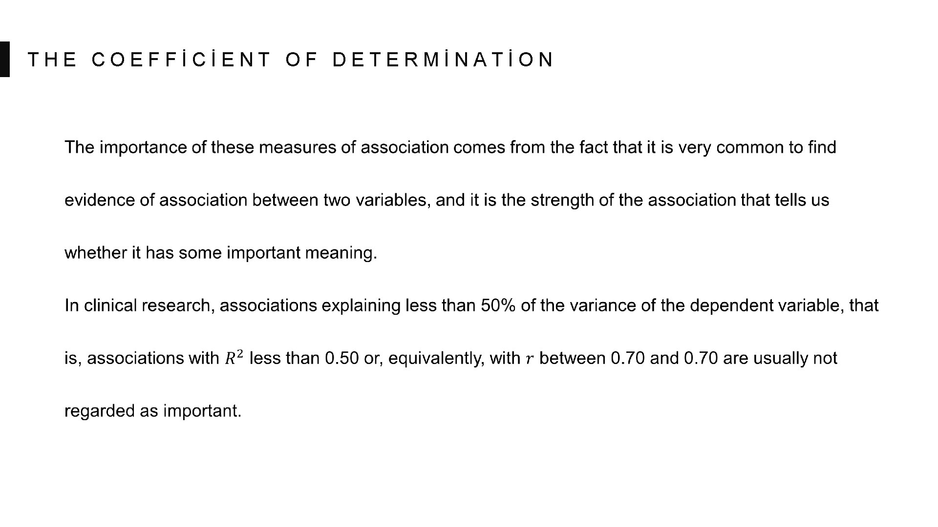
THE COEFFİCİENT OF DETERMİNATİON

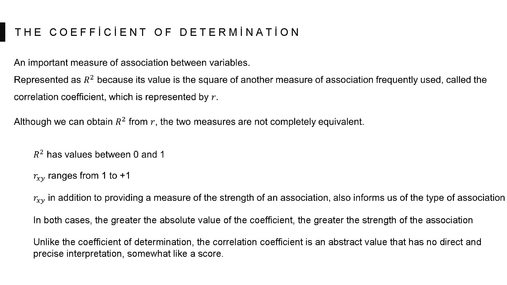
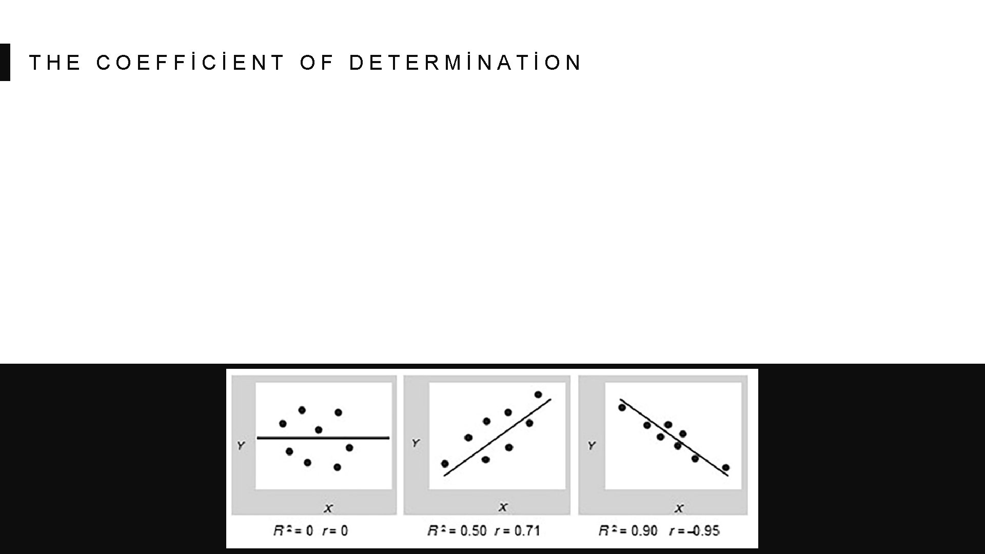
THE COEFFİCİENT OF DETERMİNATİON In both cases, the greater the absolute value of the coefficient, the greater the strength of the association Unlike the coefficient of determination, the correlation coefficient is an abstract value that has no direct and precise interpretation, somewhat like a score.

THE COEFFİCİENT OF DETERMİNATİON

THE COEFFİCİENT OF DETERMİNATİON

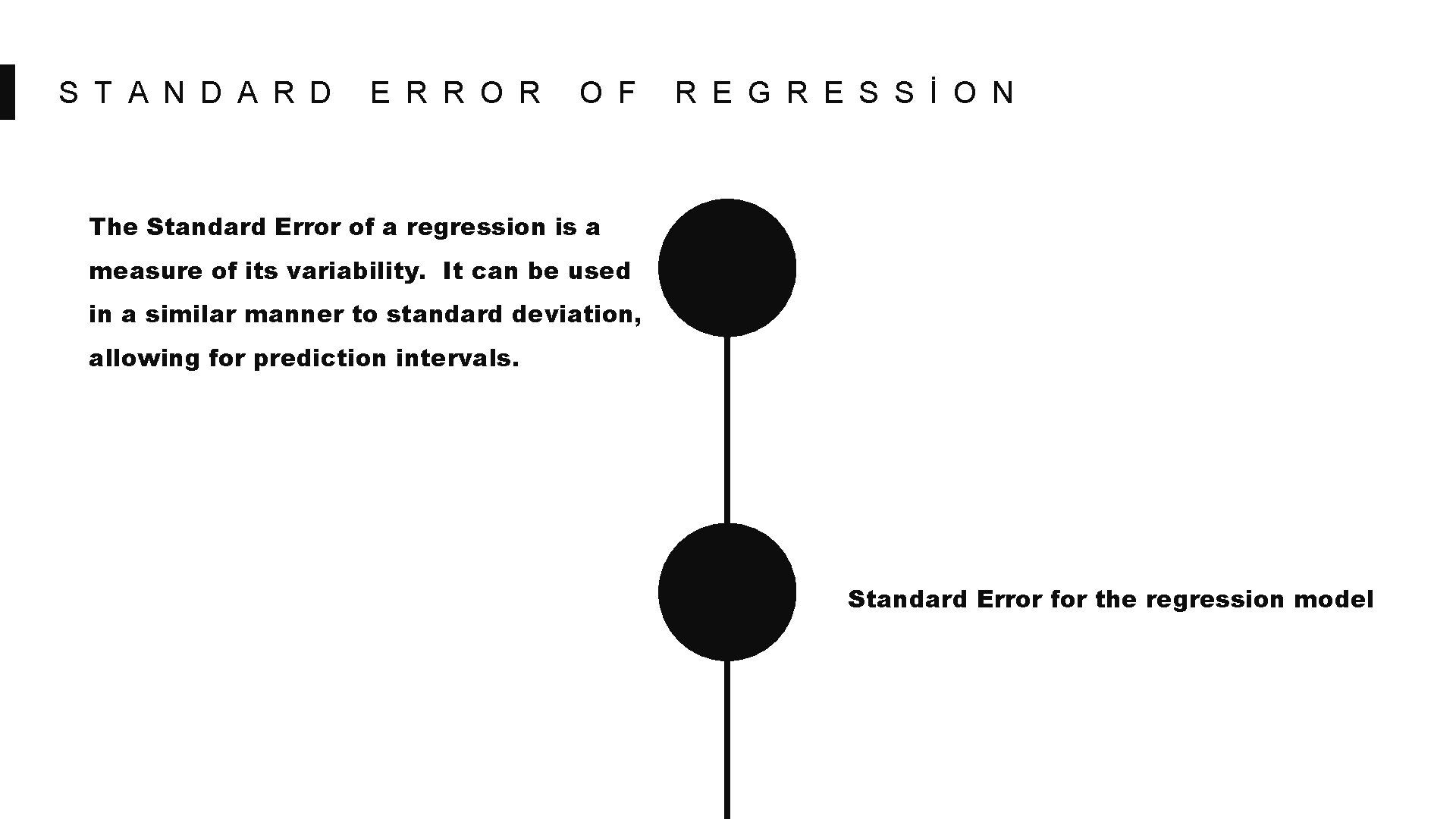
S T A N D A R D E R R O R O F R E G R E S S İ O N The Standard Error of a regression is a measure of its variability. It can be used in a similar manner to standard deviation, allowing for prediction intervals. Standard Error for the regression model

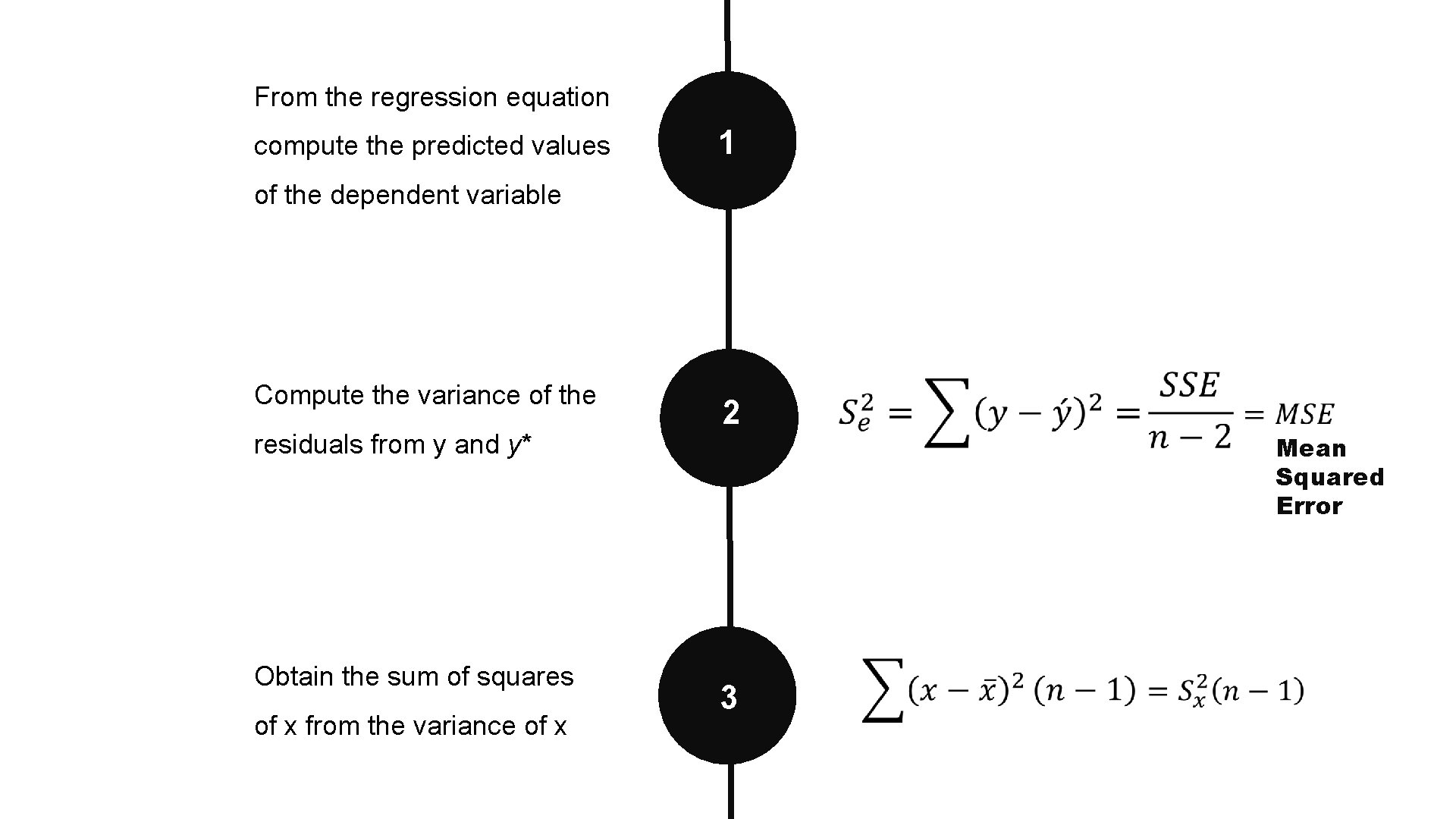
From the regression equation compute the predicted values 1 of the dependent variable Compute the variance of the residuals from y and y* Obtain the sum of squares of x from the variance of x 2 Mean Squared Error 3

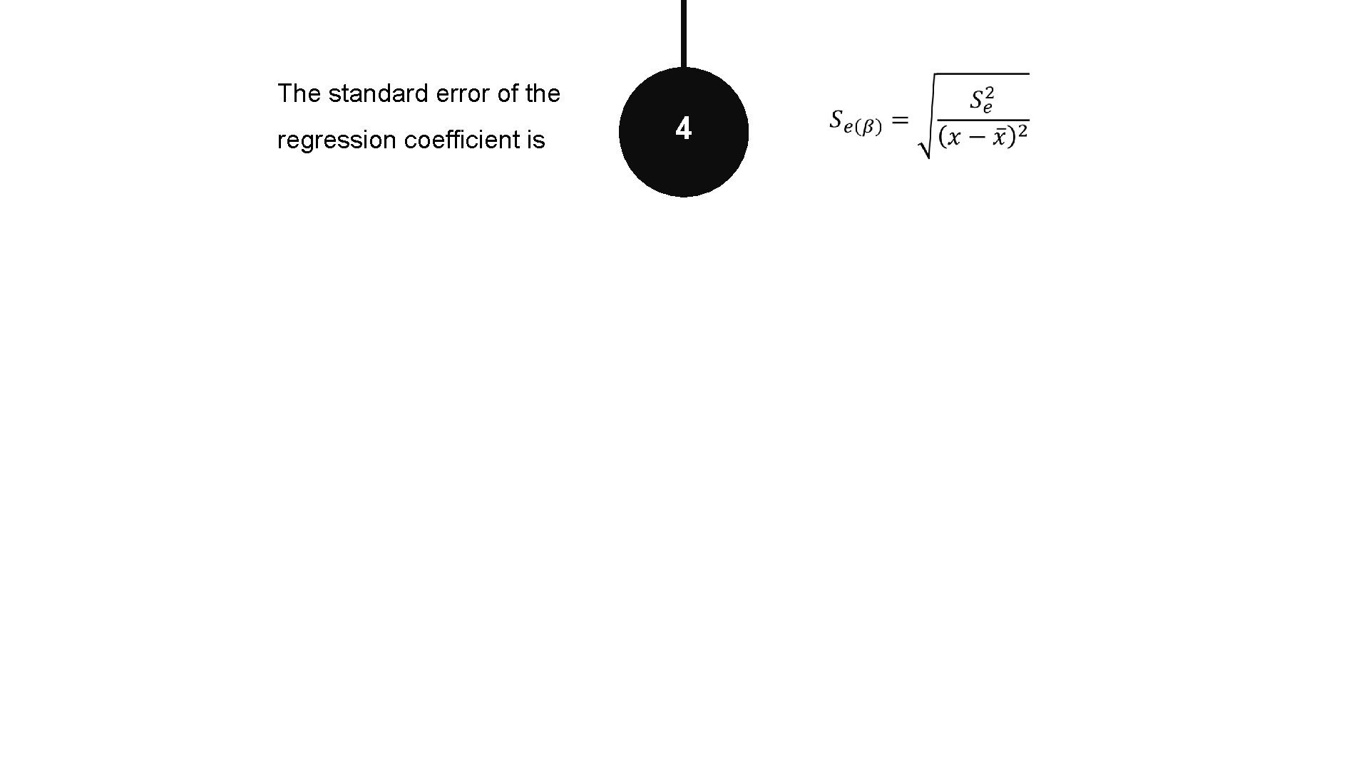
The standard error of the regression coefficient is 4

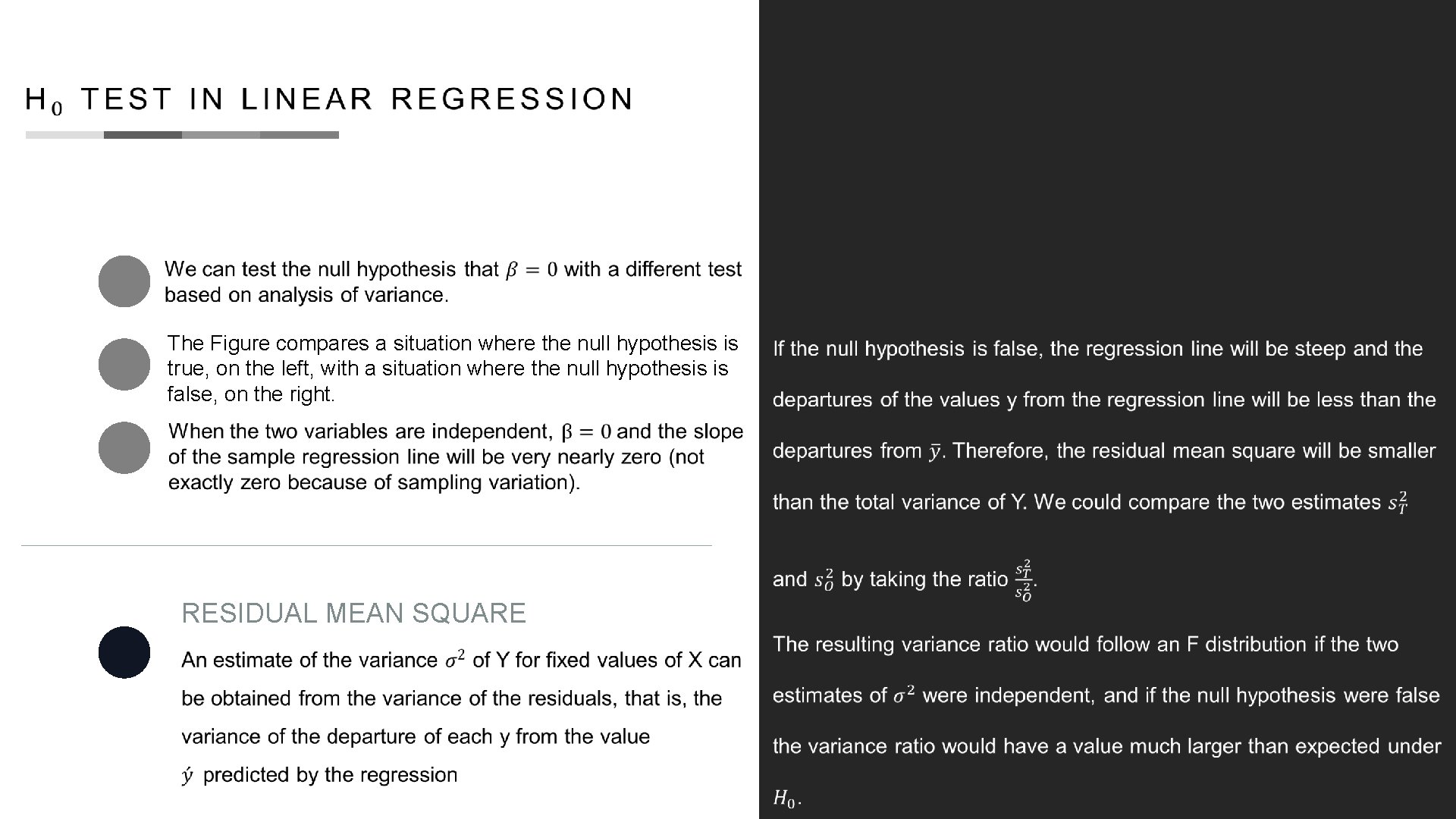
The Figure compares a situation where the null hypothesis is true, on the left, with a situation where the null hypothesis is false, on the right. � RESIDUAL MEAN SQUARE

SECTION 4 i z Q u

Q U I Z The regression line is drawn so that: A. The line goes through more points than any other possible line, straight or curved B. The line goes through more points than any other possible straight line. C. The same number of points are below and above the regression line. D. The sum of the absolute errors is as small as possible. E. The sum of the squared errors is as small as possible.

Q U I Z In order for the regression technique to give the best and minimum variance prediction, all the following conditions must be met, EXCEPT for: A. The relation is linear. B. We have not omitted any significant variable. C. Both the X and Y variables (the predictors and the response) are normally distributed. D. The residuals (errors) are normally distributed. E. The variance around the regression line is about the same for all values of the predictor. C. Both the X and Y variables (the predictors and the response) are normally distributed.

Q U I Z If a regression has the problem of heteroscedasticity, A. The predictions it makes will be wrong on average. B. The predictions it makes will be correct on average, but we will not be certain of the RMSE (root-mean-square error) C. It will also have the problem of an omitted variable or variables. D. It will also be based on a non-linear equation The assumption of homoscedasticity (meaning “same variance”) is central to linear regression models. Homoscedasticity describes a situation in which the error term (that is, the “noise” or random disturbance in the relationship between the independent variables and the dependent variable) is the same across all values of the independent variables. Heteroscedasticity (the violation of homoscedasticity) is present when the size of the error term differs across values of an independent variable. The impact of violating the assumption of homoscedasticity is a matter of degree, increasing as heteroscedasticity increases. B. Heteroscedasticity implies that the variance will differ for different values of the regressor.

Q U I Z In regression, the equation that describes how the response variable (y) is related to the explanatory variable (x) is: a. the correlation model b. the regression model c. used to compute the correlation coefficient d. None of these alternatives is correct. b. the regression model

Q U I Z The regression line is drawn so that: A. The line goes through more points than any other possible line, straight or curved B. The line goes through more points than any other possible straight line. C. The same number of points are below and above the regression line. D. The sum of the absolute errors is as small as possible. E. The sum of the squared errors is as small as possible.

Q U I Z The relationship between number of beers consumed (x) and blood alcohol content (y) was studied in 16 male college students by using least squares regression. The following regression equation was obtained from this study: y= -0. 0127 + 0. 0180 x The above equation implies that: a. each beer consumed increases blood alcohol by 1. 27% b. on average it takes 1. 8 beers to increase blood alcohol content by 1% c. each beer consumed increases blood alcohol by an average of amount of 1. 8% d. each beer consumed increases blood alcohol by exactly 0. 018 c. each beer consumed increases blood alcohol by an average of amount of 1. 8%

Q U I Z SSE can never be a. larger than SST b. smaller than SST c. equal to 1 d. equal to zero a. larger than SST

Q U I Z Regression modeling is a statistical framework for developing a mathematical equation that describes how a. one explanatory and one or more response variables are related b. several explanatory and several response variables response are related c. one response and one or more explanatory variables are related d. All of these are correct. c. one response and one or more explanatory variables are related

Q U I Z In regression analysis, the variable that is being predicted is the a. response, or dependent, variable b. independent variable c. intervening variable d. is usually x a. response, or dependent, variable

Q U I Z In least squares regression, which of the following is not a required assumption about the error term ε? a. The expected value of the error term is one. b. The variance of the error term is the same for all values of x. c. The values of the error term are independent. d. The error term is normally distributed. a. The expected value of the error term is one.

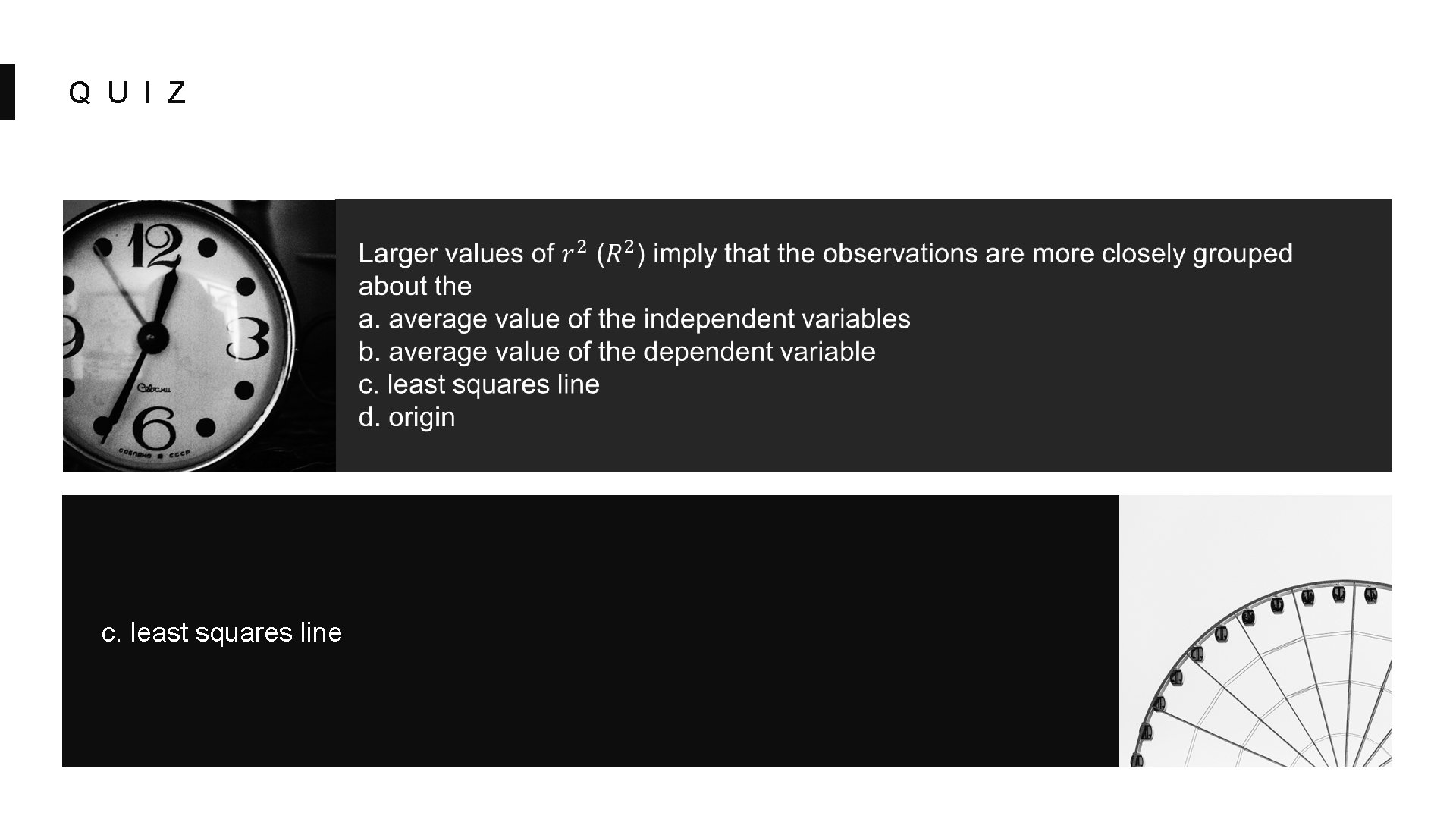
Q U I Z c. least squares line

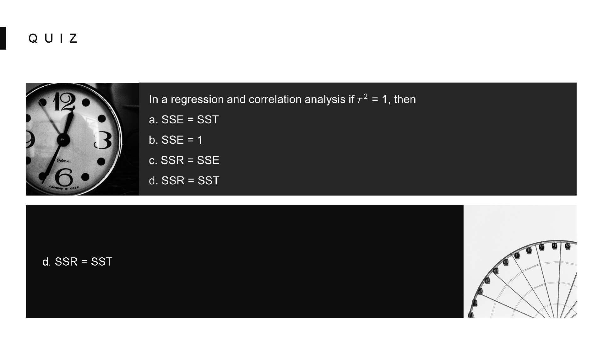
Q U I Z In a regression analysis if r 2 = 1, then a. SSE must also be equal to one b. SSE must be equal to zero c. SSE can be any positive value d. SSE must be negative b. SSE must be equal to zero

Q U I Z In regression analysis, the variable that is used to explain the change in the outcome of an experiment, or some natural process, is called a. the x-variable b. the independent variable c. the predictor variable d. the explanatory variable e. all of the above (a-d) are correct f. none are correct e. all of the above (a-d) are correct

Q U I Z In the case of an algebraic model for a straight line, if a value for the x variable is specified, then a. the exact value of the response variable can be computed b. the computed response to the independent value will always give a minimal residual c. the computed value of y will always be the best estimate of the mean response d. none of these alternatives is correct. a. the exact value of the response variable can be computed

Q U I Z d. SSR = SST

Q U I Z If the coefficient of determination is a positive value, then the regression equation a. must have a positive slope b. must have a negative slope c. could have either a positive or a negative slope d. must have a positive y intercept c. could have either a positive or a negative slope

Q U I Z If two variables, x and y, have a very strong linear relationship, then a. there is evidence that x causes a change in y b. there is evidence that y causes a change in x c. there might not be any causal relationship between x and y d. None of these alternatives is correct. c. there might not be any causal relationship between x and y

Q U I Z In regression analysis, if the independent variable is measured in kilograms, the dependent variable a. must also be in kilograms b. must be in some unit of weight c. cannot be in kilograms d. can be any units

Q U I Z In a regression analysis if SSE = 200 and SSR = 300, then the coefficient of determination is a. 0. 6667 b. 0. 6000 c. 0. 4000 d. 1. 5000 b. 0. 6000

Q U I Z A fitted least squares regression line a. may be used to predict a value of y if the corresponding x value is given b. is evidence for a cause-effect relationship between x and y c. can only be computed if a strong linear relationship exists between x and y d. None of these alternatives is correct. a. may be used to predict a value of y if the corresponding x value is given

Q U I Z You have carried out a regression analysis; but, after thinking about the relationship between variables, you have decided you must swap the explanatory and the response variables. After refitting the regression model to the data you expect that: a. the value of the correlation coefficient will change b. the value of SSE will change c. the value of the coefficient of determination will change d. the sign of the slope will change e. nothing changes b. the value of SSE will change

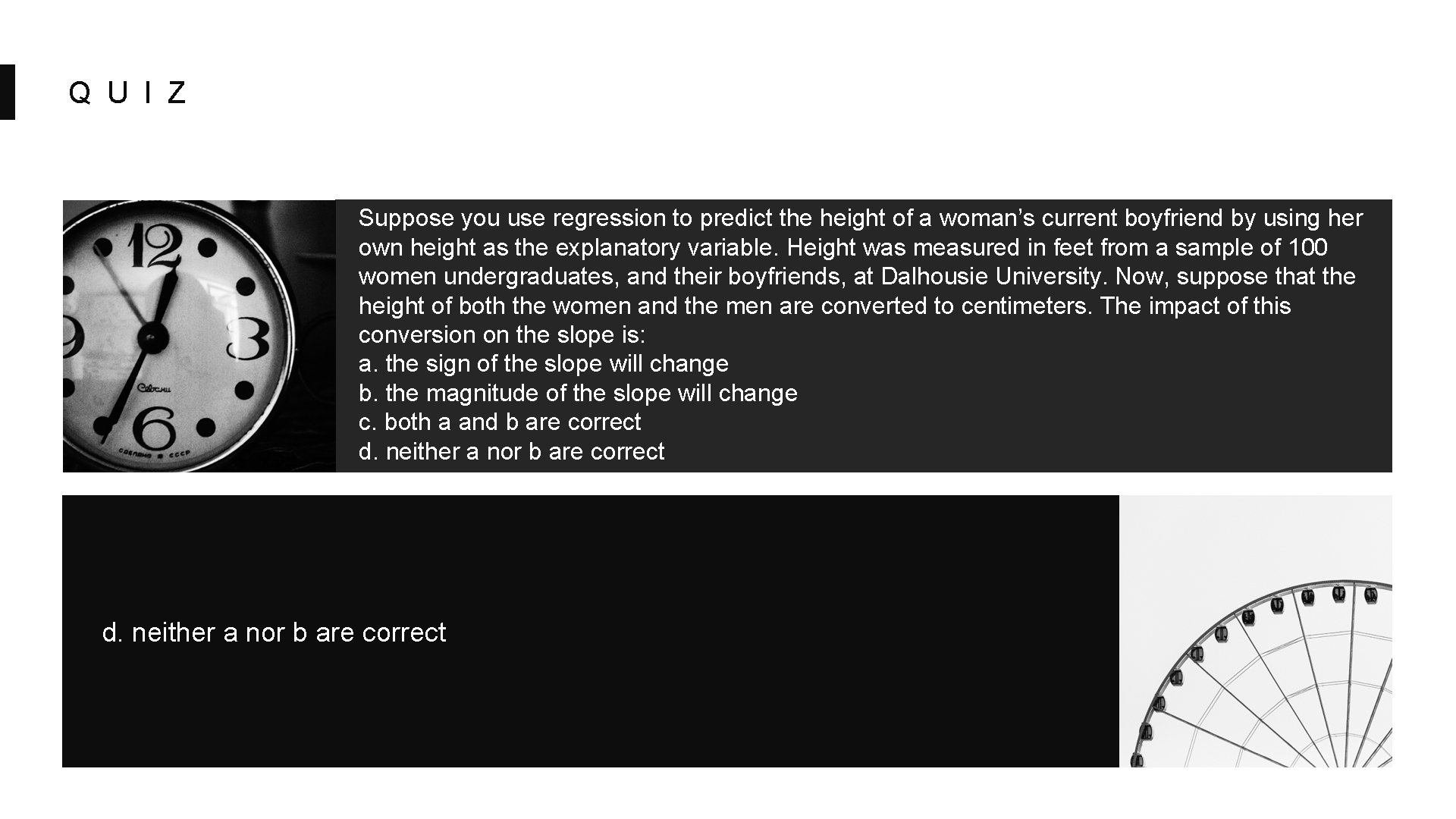
Q U I Z Suppose you use regression to predict the height of a woman’s current boyfriend by using her own height as the explanatory variable. Height was measured in feet from a sample of 100 women undergraduates, and their boyfriends, at Dalhousie University. Now, suppose that the height of both the women and the men are converted to centimeters. The impact of this conversion on the slope is: a. the sign of the slope will change b. the magnitude of the slope will change c. both a and b are correct d. neither a nor b are correct

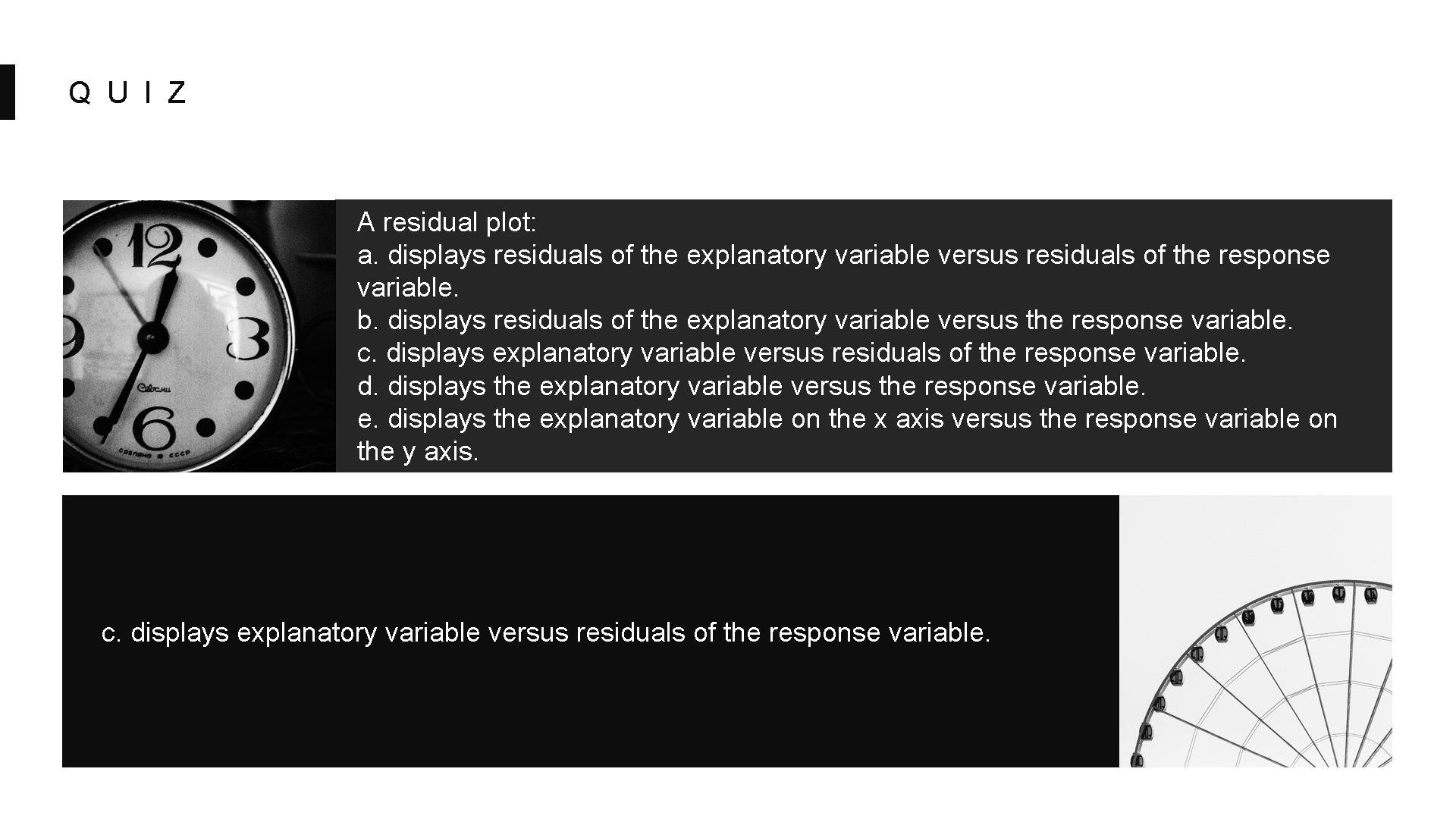
Q U I Z A residual plot: a. displays residuals of the explanatory variable versus residuals of the response variable. b. displays residuals of the explanatory variable versus the response variable. c. displays explanatory variable versus residuals of the response variable. d. displays the explanatory variable versus the response variable. e. displays the explanatory variable on the x axis versus the response variable on the y axis. c. displays explanatory variable versus residuals of the response variable.

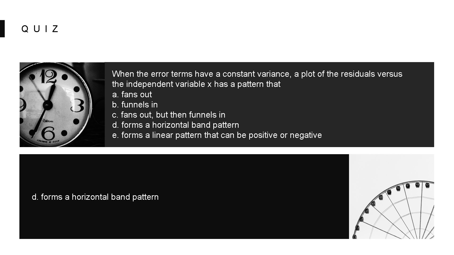
Q U I Z When the error terms have a constant variance, a plot of the residuals versus the independent variable x has a pattern that a. fans out b. funnels in c. fans out, but then funnels in d. forms a horizontal band pattern e. forms a linear pattern that can be positive or negative d. forms a horizontal band pattern

THANK YOU S E R V E R. R A R E D I S. O R G / E D U