Queuing Theory Simulation Modeling The Queuing Model Queuing

Queuing Theory Simulation & Modeling

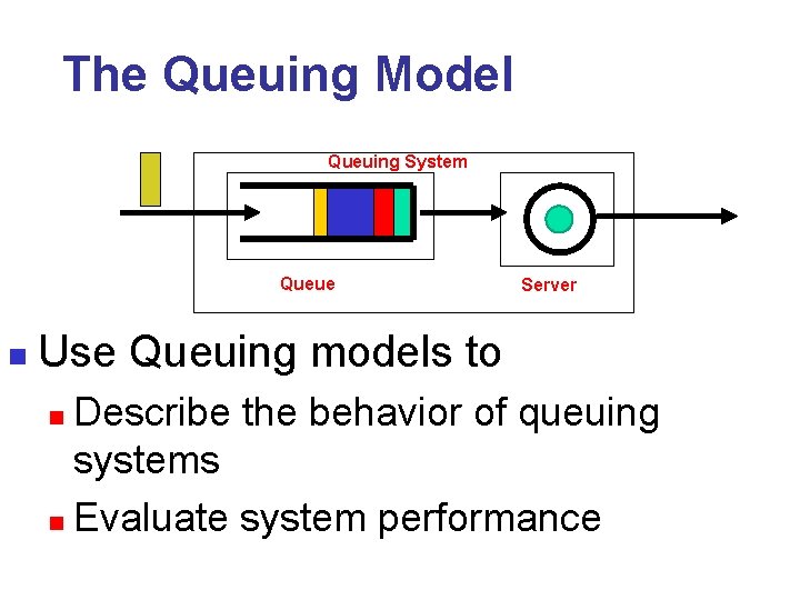
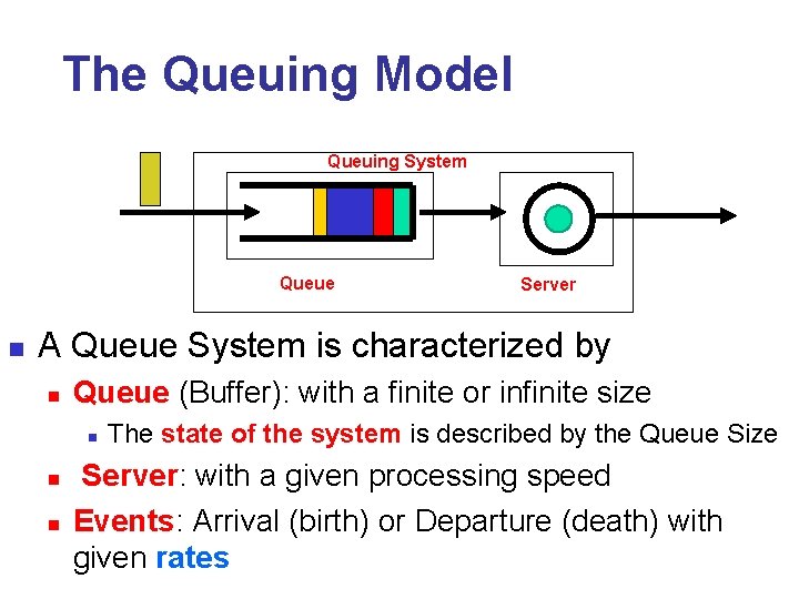
The Queuing Model Queuing System Queue n Server Use Queuing models to Describe the behavior of queuing systems n Evaluate system performance n

Applications of Queuing Theory 3 n Telecommunications n Computer Networks n Predicting computer performance n Health services (eg. control of hospital bed assignments) n Airport traffic, airline ticket sales n Layout of manufacturing systems.

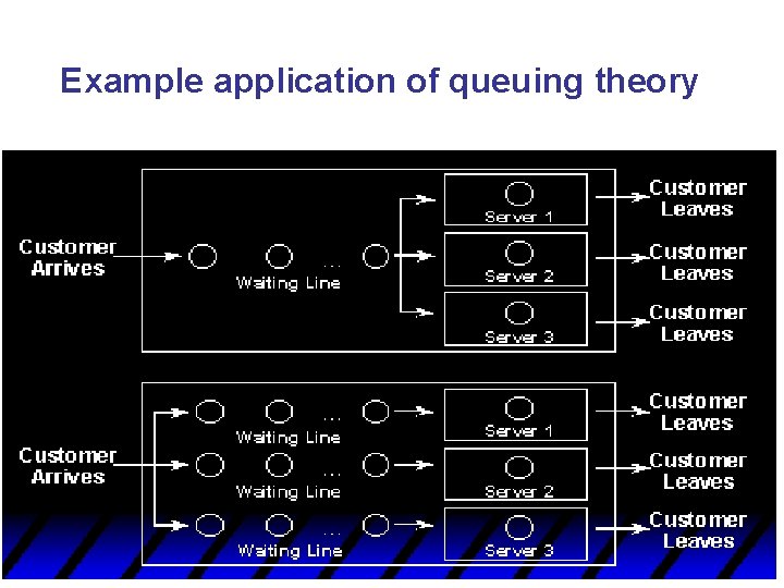
Example application of queuing theory 4 n In many stores and banks, we can find: n multiple line/multiple checkout system → a queuing system where customers wait for the next available cashier n We can prove using queuing theory that : throughput improves/increases when queues are used instead of separate lines

The Queuing Model Queuing System Queue n Server A Queue System is characterized by n Queue (Buffer): with a finite or infinite size n n n The state of the system is described by the Queue Size Server: with a given processing speed Events: Arrival (birth) or Departure (death) with given rates

Example application of queuing theory 6

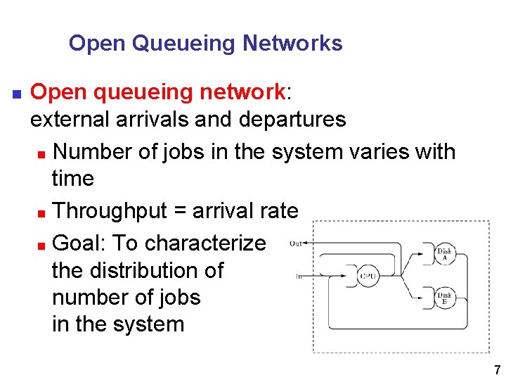
Open Queueing Networks n Open queueing network: external arrivals and departures n Number of jobs in the system varies with time n Throughput = arrival rate n Goal: To characterize the distribution of number of jobs in the system 7

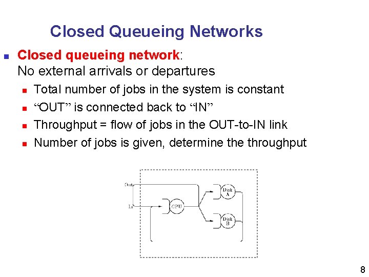
Closed Queueing Networks n Closed queueing network: No external arrivals or departures n n Total number of jobs in the system is constant “OUT” is connected back to “IN” Throughput = flow of jobs in the OUT-to-IN link Number of jobs is given, determine throughput 8

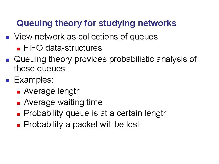
Queuing theory for studying networks 9 n n n View network as collections of queues n FIFO data-structures Queuing theory provides probabilistic analysis of these queues Examples: n Average length n Average waiting time n Probability queue is at a certain length n Probability a packet will be lost

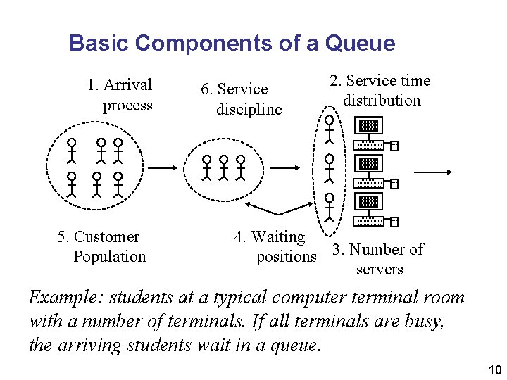
Basic Components of a Queue 1. Arrival process 5. Customer Population 6. Service discipline 2. Service time distribution 4. Waiting positions 3. Number of servers Example: students at a typical computer terminal room with a number of terminals. If all terminals are busy, the arriving students wait in a queue. 10

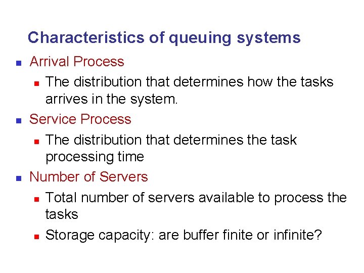
Characteristics of queuing systems 11 n n n Arrival Process n The distribution that determines how the tasks arrives in the system. Service Process n The distribution that determines the task processing time Number of Servers n Total number of servers available to process the tasks n Storage capacity: are buffer finite or infinite?

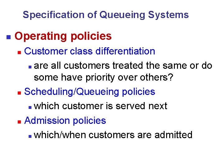
Specification of Queueing Systems n Operating policies Customer class differentiation n are all customers treated the same or do some have priority over others? n Scheduling/Queueing policies n which customer is served next n Admission policies n which/when customers are admitted n

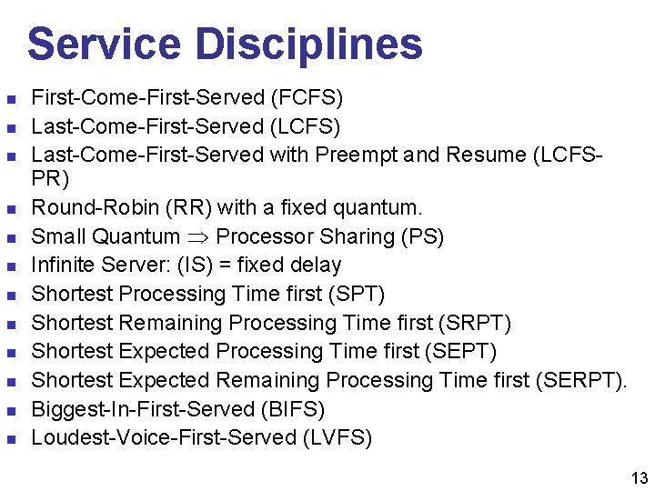
Service Disciplines n n n First-Come-First-Served (FCFS) Last-Come-First-Served (LCFS) Last-Come-First-Served with Preempt and Resume (LCFSPR) Round-Robin (RR) with a fixed quantum. Small Quantum Processor Sharing (PS) Infinite Server: (IS) = fixed delay Shortest Processing Time first (SPT) Shortest Remaining Processing Time first (SRPT) Shortest Expected Processing Time first (SEPT) Shortest Expected Remaining Processing Time first (SERPT). Biggest-In-First-Served (BIFS) Loudest-Voice-First-Served (LVFS) 13

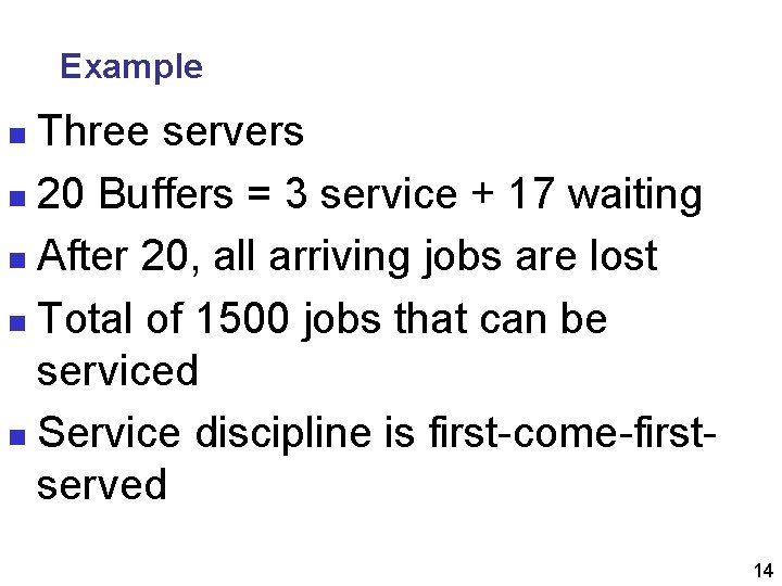
Example Three servers n 20 Buffers = 3 service + 17 waiting n After 20, all arriving jobs are lost n Total of 1500 jobs that can be serviced n Service discipline is first-come-firstserved n 14

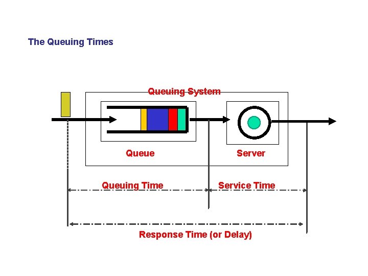
The Queuing Times Queuing System Queue Queuing Time Server Service Time Response Time (or Delay)

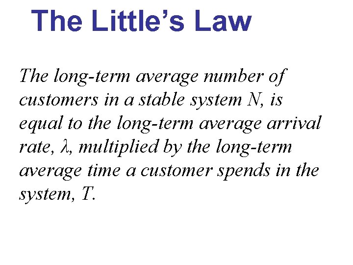
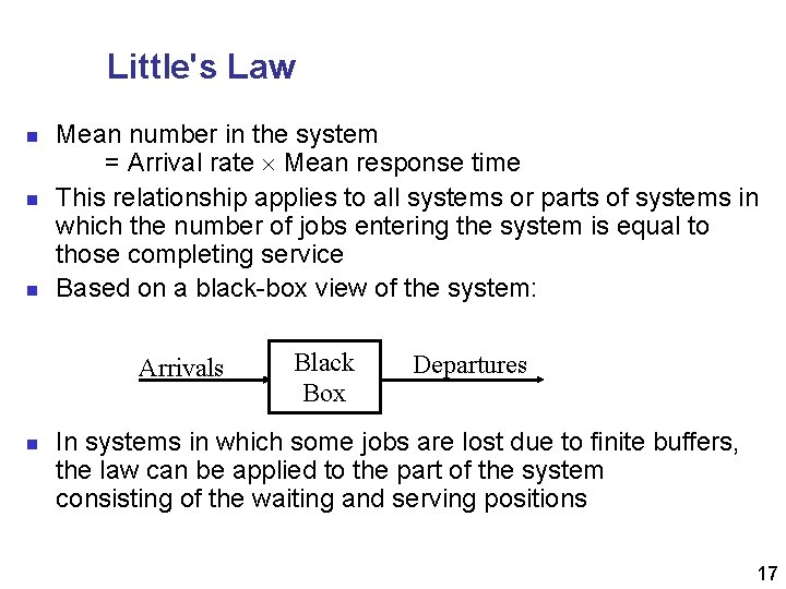
The Little’s Law The long-term average number of customers in a stable system N, is equal to the long-term average arrival rate, λ, multiplied by the long-term average time a customer spends in the system, T.

Little's Law n n n Mean number in the system = Arrival rate Mean response time This relationship applies to all systems or parts of systems in which the number of jobs entering the system is equal to those completing service Based on a black-box view of the system: Arrivals n Black Box Departures In systems in which some jobs are lost due to finite buffers, the law can be applied to the part of the system consisting of the waiting and serving positions 17

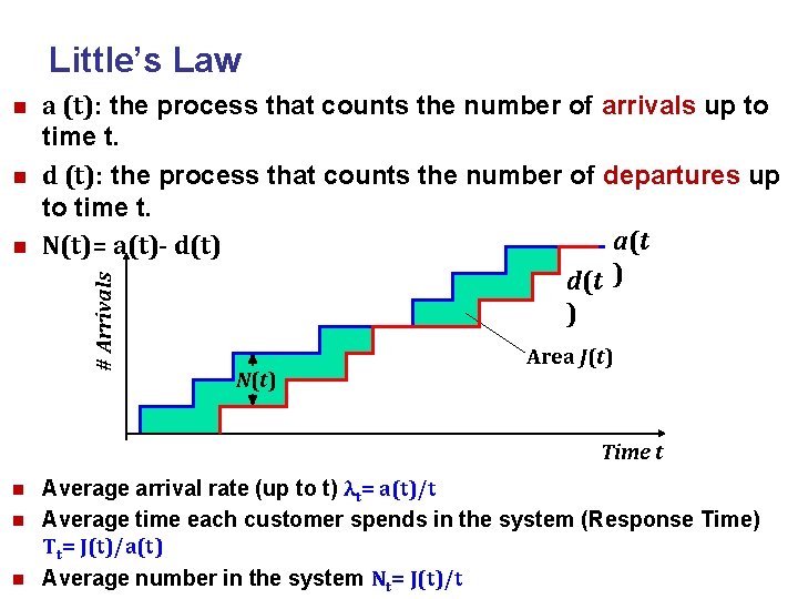
Little’s Law n n # Arrivals n a (t): the process that counts the number of arrivals up to time t. d (t): the process that counts the number of departures up to time t. a(t N(t)= a(t)- d(t) d(t ) ) N(t) Area J(t) Time t n n n Average arrival rate (up to t) λt= a(t)/t Average time each customer spends in the system (Response Time) Tt= J(t)/a(t) Average number in the system Nt= J(t)/t

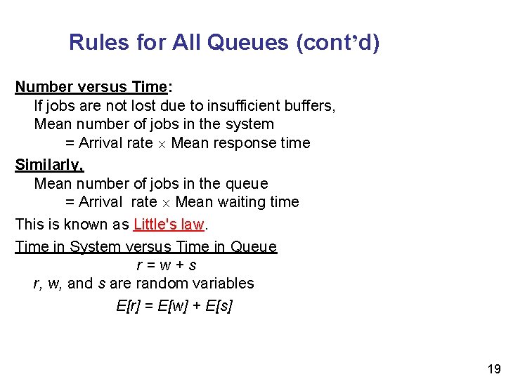
Rules for All Queues (cont’d) Number versus Time: If jobs are not lost due to insufficient buffers, Mean number of jobs in the system = Arrival rate Mean response time Similarly, Mean number of jobs in the queue = Arrival rate Mean waiting time This is known as Little's law. Time in System versus Time in Queue r=w+s r, w, and s are random variables E[r] = E[w] + E[s] 19

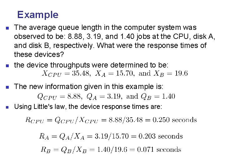
Example n The average queue length in the computer system was observed to be: 8. 88, 3. 19, and 1. 40 jobs at the CPU, disk A, and disk B, respectively. What were the response times of these devices? the device throughputs were determined to be: n The new information given in this example is: n Using Little's law, the device response times are: n

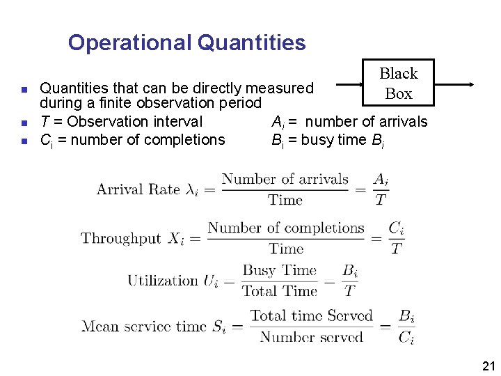
Operational Quantities n n n Black Box Quantities that can be directly measured during a finite observation period T = Observation interval Ai = number of arrivals Ci = number of completions Bi = busy time Bi 21

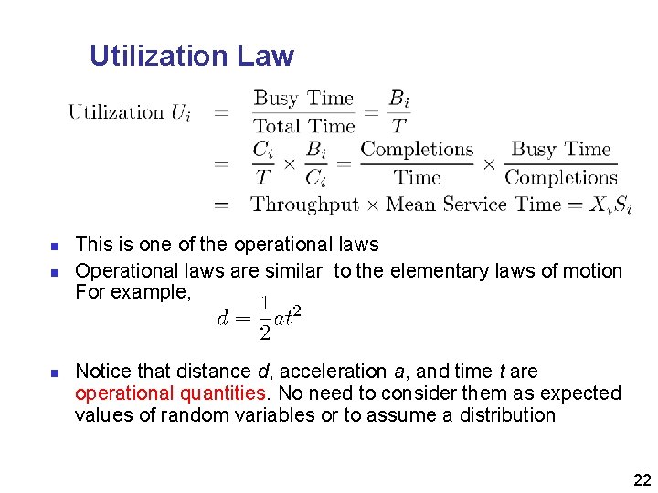
Utilization Law n n n This is one of the operational laws Operational laws are similar to the elementary laws of motion For example, Notice that distance d, acceleration a, and time t are operational quantities. No need to consider them as expected values of random variables or to assume a distribution 22

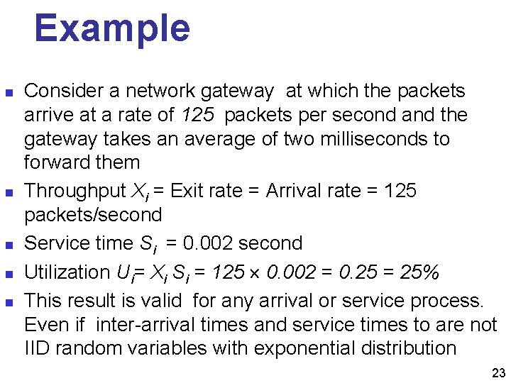
Example n n n Consider a network gateway at which the packets arrive at a rate of 125 packets per second and the gateway takes an average of two milliseconds to forward them Throughput Xi = Exit rate = Arrival rate = 125 packets/second Service time Si = 0. 002 second Utilization Ui= Xi Si = 125 0. 002 = 0. 25 = 25% This result is valid for any arrival or service process. Even if inter-arrival times and service times to are not IID random variables with exponential distribution 23

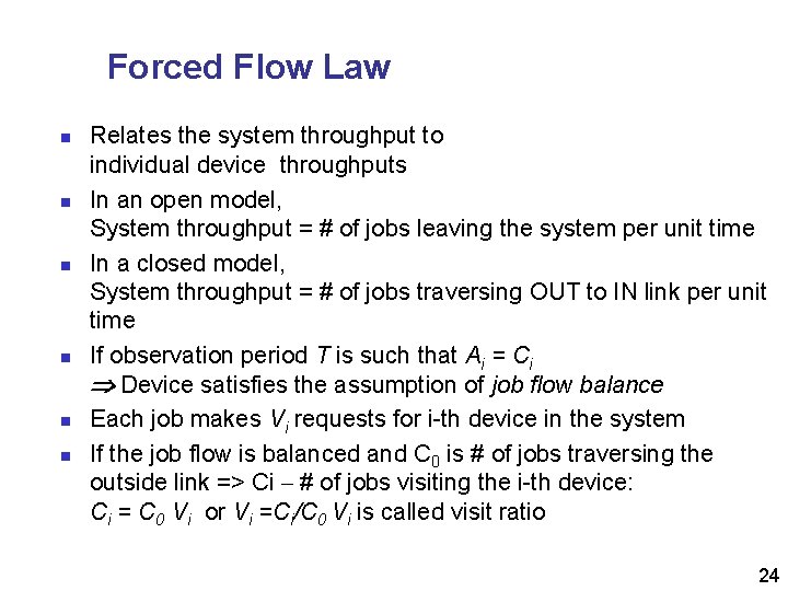
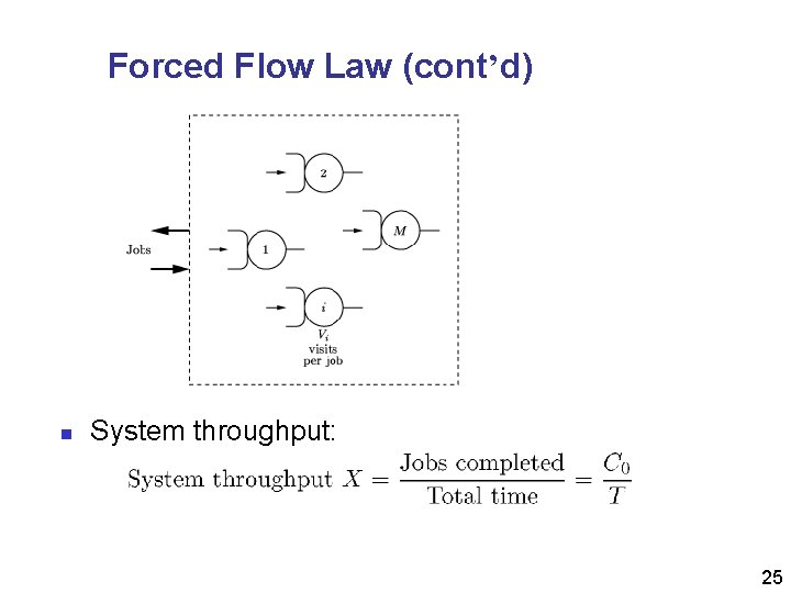
Forced Flow Law n n n Relates the system throughput to individual device throughputs In an open model, System throughput = # of jobs leaving the system per unit time In a closed model, System throughput = # of jobs traversing OUT to IN link per unit time If observation period T is such that Ai = Ci Device satisfies the assumption of job flow balance Each job makes Vi requests for i-th device in the system If the job flow is balanced and C 0 is # of jobs traversing the outside link => Ci – # of jobs visiting the i-th device: Ci = C 0 Vi or Vi =Ci/C 0 Vi is called visit ratio 24

Forced Flow Law (cont’d) n System throughput: 25

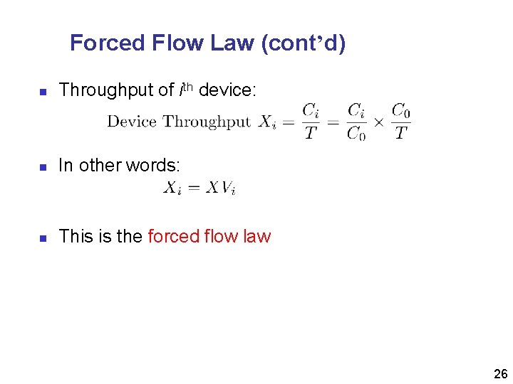
Forced Flow Law (cont’d) n Throughput of ith device: n In other words: n This is the forced flow law 26

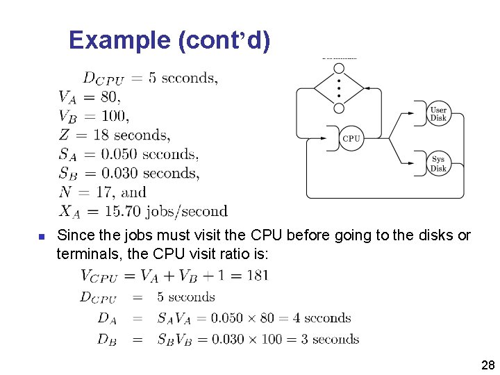
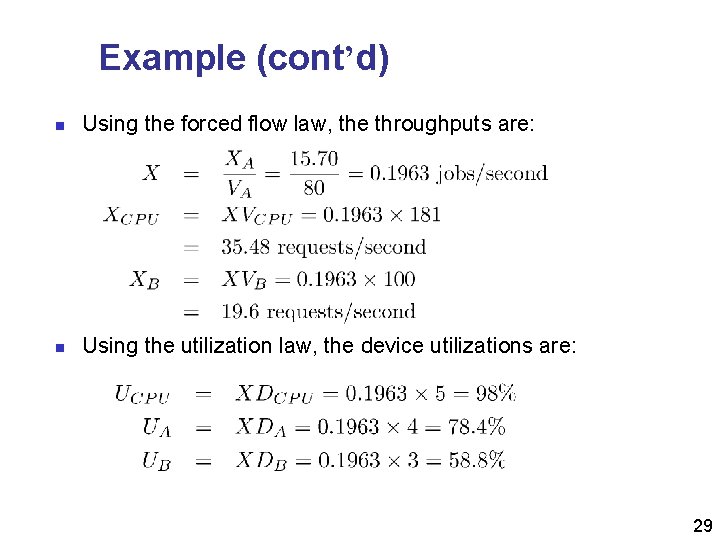
Example n n In a timesharing system, accounting log data produced the following profile for user programs n Each program requires five seconds of CPU time, makes 80 I/O requests to the disk A and 100 I/O requests to disk B n Average think-time of the users was 18 seconds n From the device specifications, it was determined that disk A takes 50 milliseconds to satisfy an I/O request and the disk B takes 30 milliseconds per request n With 17 active terminals, disk A throughput was observed to be 15. 70 I/O requests per second We want to find the system throughput and device utilizations 27

Example (cont’d) n Since the jobs must visit the CPU before going to the disks or terminals, the CPU visit ratio is: 28

Example (cont’d) n Using the forced flow law, the throughputs are: n Using the utilization law, the device utilizations are: 29

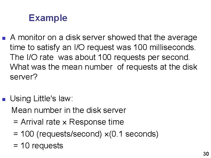
Example n n A monitor on a disk server showed that the average time to satisfy an I/O request was 100 milliseconds. The I/O rate was about 100 requests per second. What was the mean number of requests at the disk server? Using Little's law: Mean number in the disk server = Arrival rate Response time = 100 (requests/second) (0. 1 seconds) = 10 requests 30