Queuing Analysis Two analytical techniques can be employed

Queuing Analysis Two analytical techniques can be employed to study queuing processes: • Shock wave analysis – Demand-capacity process is deterministic – Suited to evaluating the space occupied by the queuing processes and their interactions • Queuing analysis – Deterministic (input-output) or stochastic – Vertical queues are assumed

Objectives 1. To estimate queuing characteristics when demand exceeds capacity at a bottleneck. For example, a. Average number of vehicles in a queue at a given time b. Average delay per vehicle c. Total hours of delay d. Duration of queuing 2. To determine idle time (of system, employees, etc. )

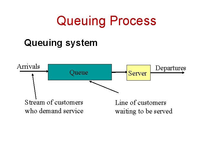
Queuing Process Queuing system Arrivals Queue Stream of customers who demand service Server Departures Line of customers waiting to be served

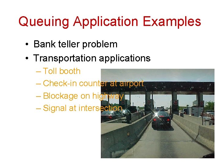
Queuing Application Examples • Bank teller problem • Transportation applications – Toll booth – Check-in counter at airport – Blockage on highway – Signal at intersection

Queuing Analysis in Traffic Applications Arrivals Queue arrival rate determined by traffic demand Server Departures departure rate determined by facility capacity How long the queue is going to be? How much delay? Duration of congestion? …

Queuing Characteristics/Classifications • • Arrivals: l (rate, distribution) Servicing: m (rate, distribution) Queue discipline: (e. g. FIFO) Number of channels (m) • Arrival rate=demand=input • Service rate=capacity=departure=output

Queue discipline • First come (in) – first served (out) (FIFO) • First in, last out (FILO) • Random service (SIRO: served in random order) • Priority • Inpatient customer • Infinite (∞)or finite lines

Queuing Models • Deterministic – Arrival and servicing are uniform (same interval, no randomness) – arrival and service rates may vary over time – Can be used to temporary blockage, temporary overloading, and periodical interruption such as signal • Stochastic – constant long-term arrival and service rates – Arrival and service conform to certain random distribution – short-term random fluctuation causes queue (even with arrival rate <service rate)

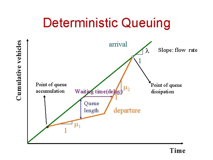
Cumulative vehicles Deterministic Queuing arrival l Slope: flow rate 1 Point of queue accumulation Waiting time(delay) Queue length 1 m 2 1 Point of queue dissipation departure m 1 Time

Deterministic Queuing Example • Vehicles arrive at the entrance to a park with a single gate where a ranger distributes a free brochure. Park opens at 8: 00 a. m. and arrivals are 480 veh/hr. After 20 min, arrival rate declines to 120 veh/hr for remainder of day. Time required to distribute a brochure is 15 seconds. • Describe operational characteristics.

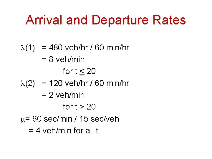
Arrival and Departure Rates l(1) = 480 veh/hr / 60 min/hr = 8 veh/min for t < 20 l(2) = 120 veh/hr / 60 min/hr = 2 veh/min for t > 20 m= 60 sec/min / 15 sec/veh = 4 veh/min for all t

Total number of vehicles 300 250 200 150 100 50 0 10 20 30 Time 40 50 60

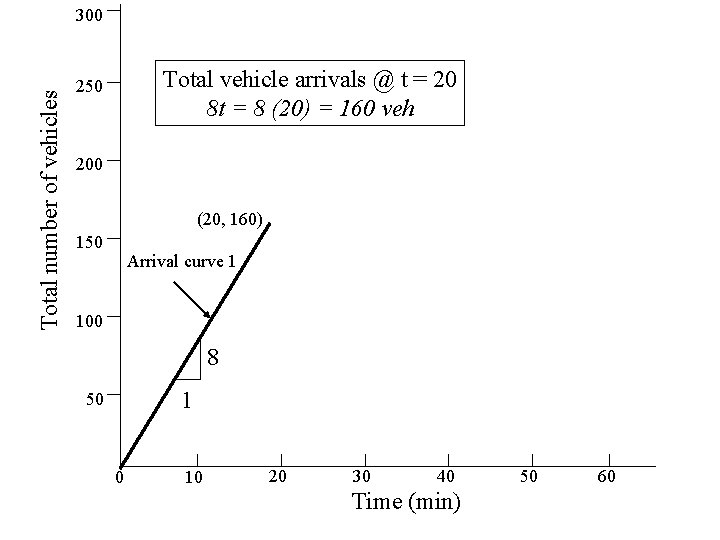
Total number of vehicles 300 Total vehicle arrivals @ t = 20 8 t = 8 (20) = 160 veh 250 200 (20, 160) 150 Arrival curve 1 100 8 1 50 0 10 20 30 40 Time (min) 50 60

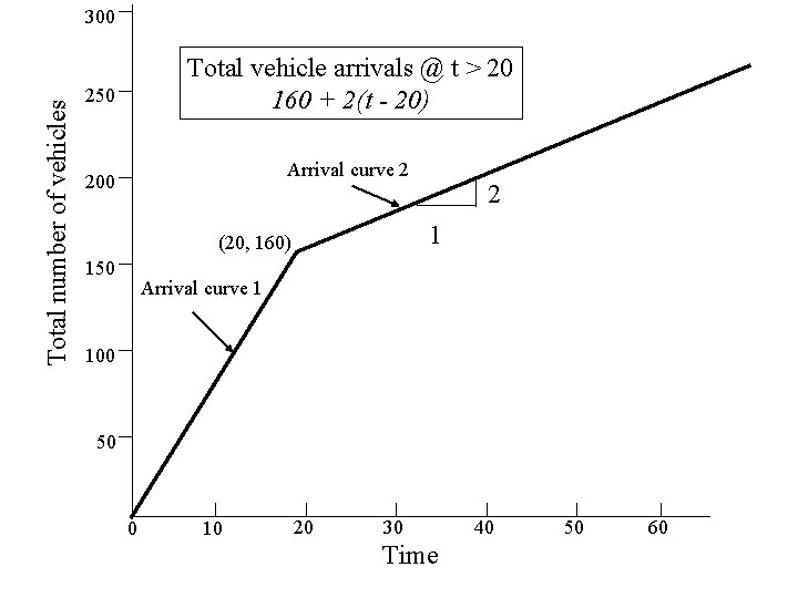
Total number of vehicles 300 Total vehicle arrivals @ t > 20 160 + 2(t - 20) 250 Arrival curve 2 200 1 (20, 160) 150 2 Arrival curve 1 100 50 0 10 20 30 Time 40 50 60

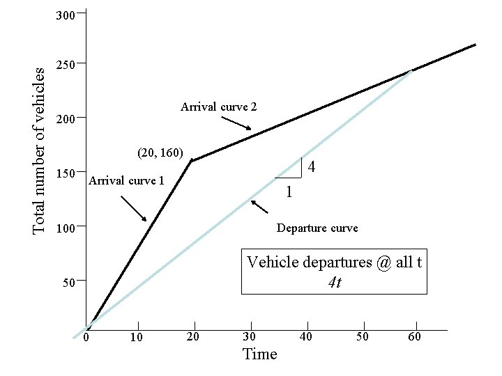
Total number of vehicles 300 250 Arrival curve 2 200 (20, 160) 150 4 Arrival curve 1 1 Departure curve 100 Vehicle departures @ all t 4 t 50 0 10 20 30 Time 40 50 60

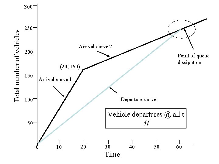
Total number of vehicles 300 250 Arrival curve 2 200 Point of queue dissipation (20, 160) 150 Arrival curve 1 Departure curve 100 Vehicle departures @ all t 4 t 50 0 10 20 30 Time 40 50 60

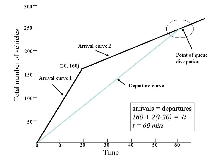
Total number of vehicles 300 250 Arrival curve 2 200 Point of queue dissipation (20, 160) 150 Arrival curve 1 Departure curve 100 arrivals = departures 160 + 2(t-20) = 4 t t = 60 min 50 0 10 20 30 Time 40 50 60

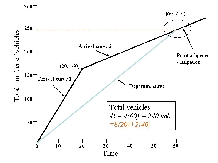
300 Total number of vehicles (60, 240) 250 Arrival curve 2 200 Point of queue dissipation (20, 160) 150 Arrival curve 1 Departure curve 100 Total vehicles 4 t = 4(60) = 240 veh =8(20)+2(40) 50 0 10 20 30 Time 40 50 60

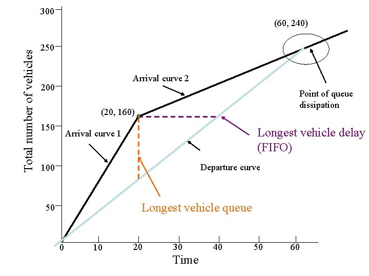
300 Total number of vehicles (60, 240) 250 Arrival curve 2 200 Point of queue dissipation (20, 160) 150 Longest vehicle delay (FIFO) Arrival curve 1 Departure curve 100 Longest vehicle queue 50 0 10 20 30 Time 40 50 60

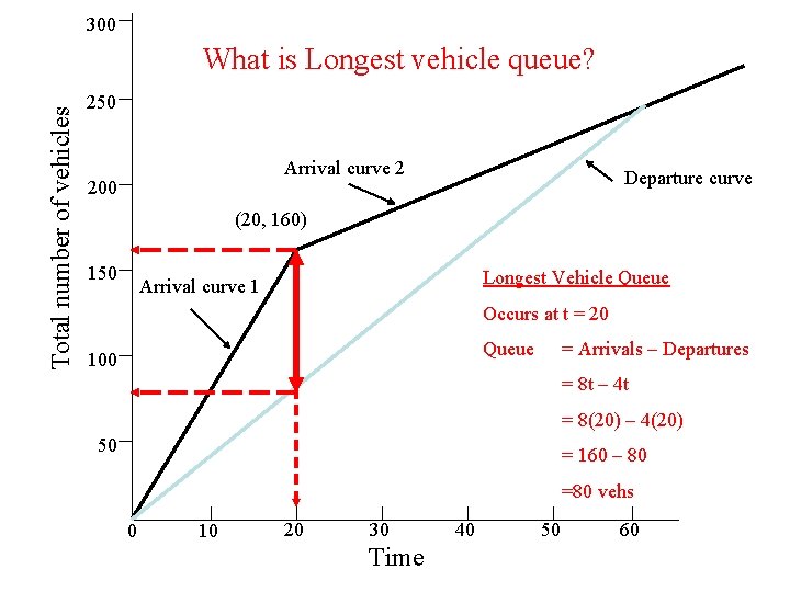
300 Total number of vehicles What is Longest vehicle queue? 250 Arrival curve 2 200 Departure curve (20, 160) 150 Longest Vehicle Queue Arrival curve 1 Occurs at t = 20 Queue 100 = Arrivals – Departures = 8 t – 4 t = 8(20) – 4(20) 50 = 160 – 80 =80 vehs 0 10 20 30 Time 40 50 60

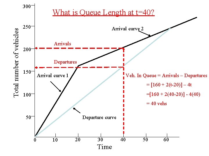
Total number of vehicles 300 What is Queue Length at t=40? 250 Arrival curve 2 Arrivals 200 Departures 150 Arrival curve 1 Veh. In Queue = Arrivals – Departures = [160 + 2(t-20)] – 4 t =[160 + 2(40 -20)] - 4(40) 100 = 40 vehs 50 Departure curve 0 10 20 30 Time 40 50 60

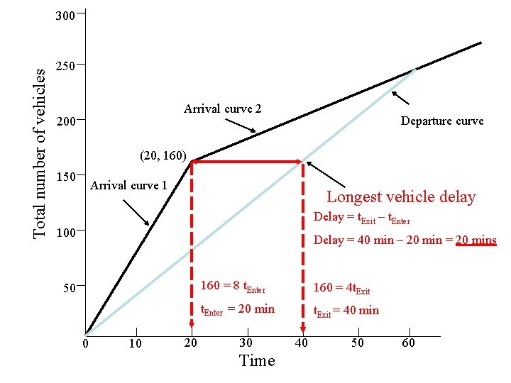
Total number of vehicles 300 250 Arrival curve 2 200 Departure curve (20, 160) 150 Arrival curve 1 Longest vehicle delay Delay = t. Exit – t. Enter 100 Delay = 40 min – 20 min = 20 mins 50 0 10 20 160 = 8 t. Enter 160 = 4 t. Exit t. Enter = 20 min t. Exit = 40 min 30 Time 40 50 60

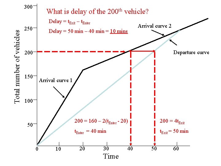
300 What is delay of the 200 th vehicle? Total number of vehicles Delay = t. Exit – t. Enter 250 Delay = 50 min – 40 min = 10 mins Arrival curve 2 Departure curve 200 150 Arrival curve 1 100 50 0 10 200 = 160 – 2(t. Enter - 20) 200 = 4 t. Exit t. Enter = 40 min t. Exit = 50 min 20 30 Time 40 50 60

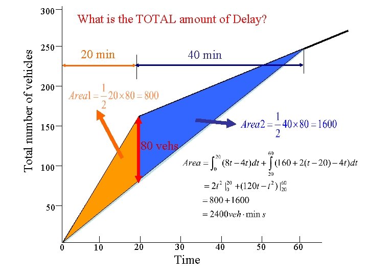
Total number of vehicles 300 What is the TOTAL amount of Delay? 250 20 min 40 min 200 150 80 vehs 100 50 0 10 20 30 Time 40 50 60

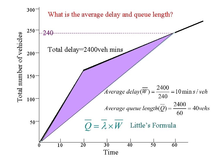
Total number of vehicles 300 What is the average delay and queue length? 250 240 Total delay=2400 veh mins 200 150 100 50 Little’s Formula 0 10 20 30 Time 40 50 60

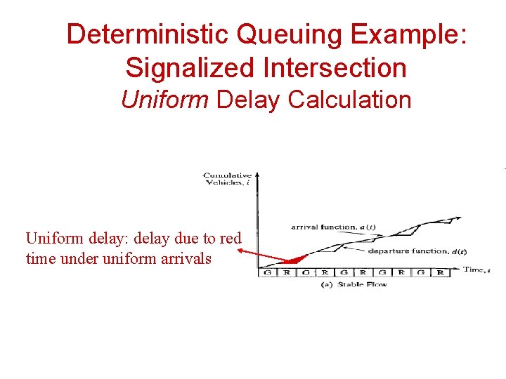
Deterministic Queuing Example: Signalized Intersection Uniform Delay Calculation Uniform delay: delay due to red time under uniform arrivals

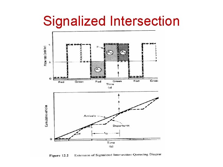
Signalized Intersection

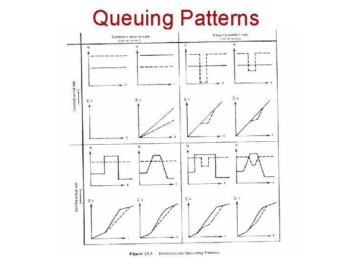
Queuing Patterns

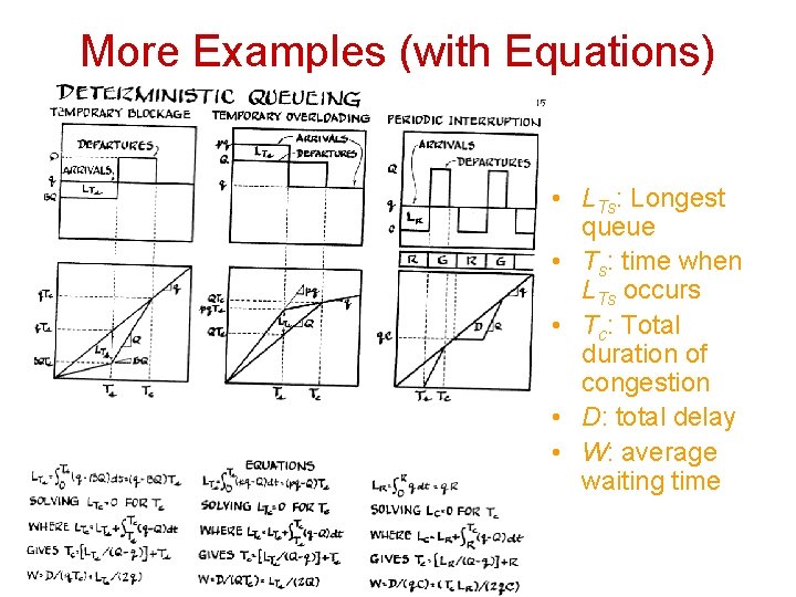
More Examples (with Equations) • LTs: Longest queue • Ts: time when LTs occurs • Tc: Total duration of congestion • D: total delay • W: average waiting time

Microscopic Analysis • Deterministic queuing analysis can be undertaken at the microscopic level • Requires arrival and departure times of individual vehicles • Computer simulation often used to calculate MOEs

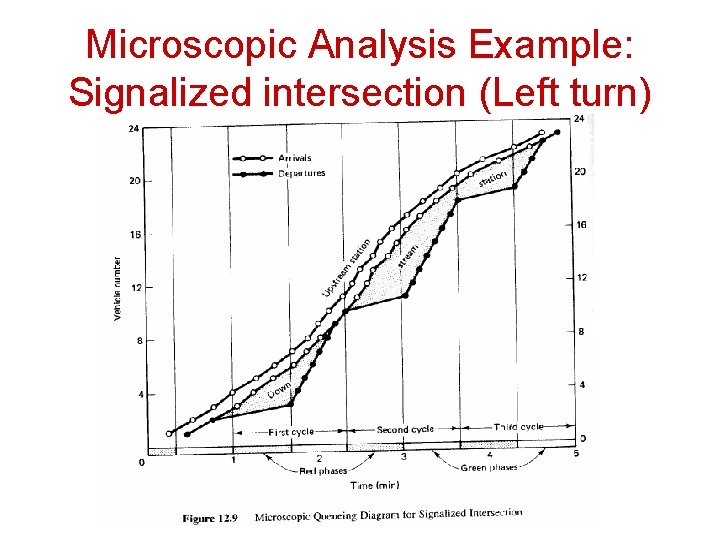
Microscopic Analysis Example: Signalized intersection (Left turn)

Stochastic Queuing Kendall’s notation Letter 1 / Letter 2 / Number – Letter 1: arrivals process – Letter 2: service process – Number of channels (servers)

Stochastic Queuing Traffic Density • ρ = λ/µ, where ρ < 1 (λ < µ) • ρ = traffic intensity • λ = mean arrival rate (vehicles per time interval) • µ = mean service rate per channel (vehicles per time interval) • λ and µ must have the same units

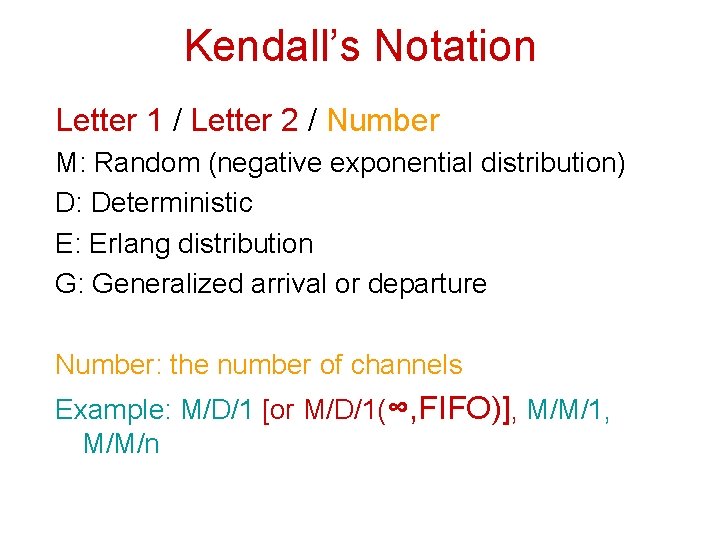
Kendall’s Notation Letter 1 / Letter 2 / Number M: Random (negative exponential distribution) D: Deterministic E: Erlang distribution G: Generalized arrival or departure Number: the number of channels Example: M/D/1 [or M/D/1(∞, FIFO)], M/M/1, M/M/n

M/D/1 Queuing Regime • Arrival times are exponentially distributed (arrivals on Poisson distribution) • Service rate deterministic (no random variation) • One service channel

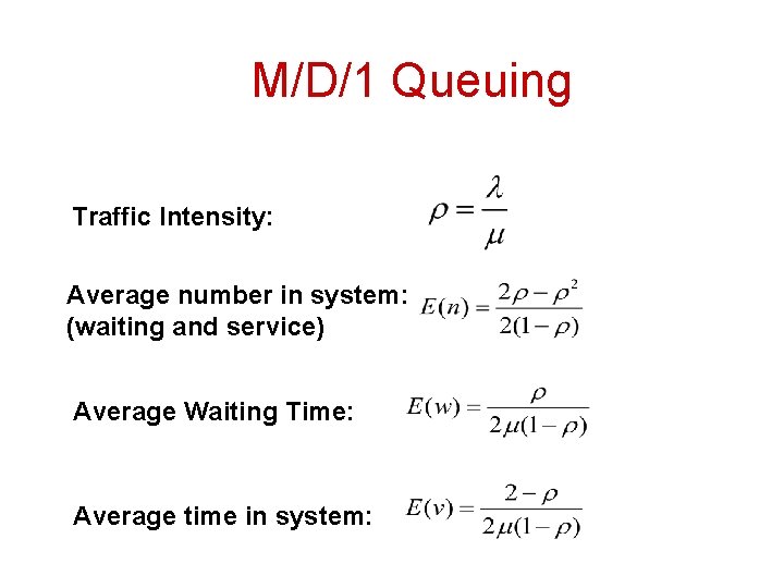
M/D/1 Queuing Traffic Intensity: Average number in system: (waiting and service) Average Waiting Time: Average time in system:

M/M/1 Queuing • Arrivals and departures are exponentially distributed • One service channel

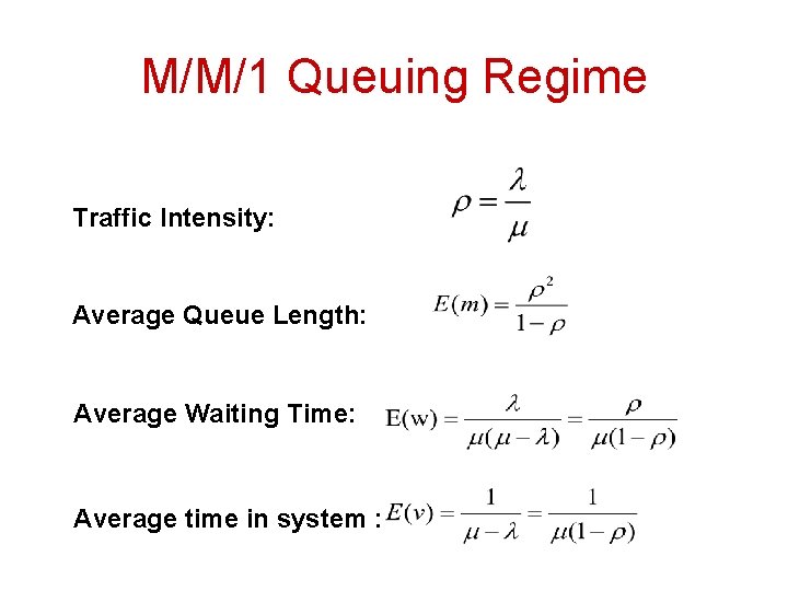
M/M/1 Queuing Regime Traffic Intensity: Average Queue Length: Average Waiting Time: Average time in system :

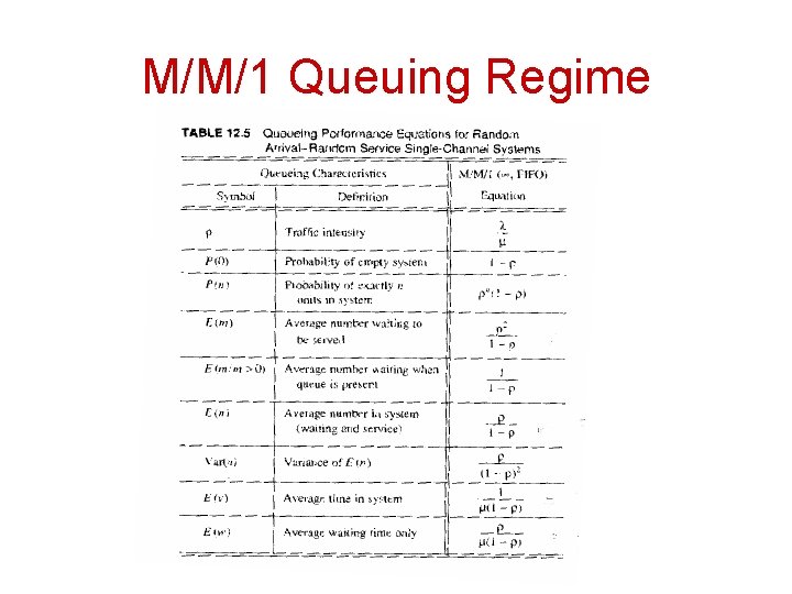
M/M/1 Queuing Regime

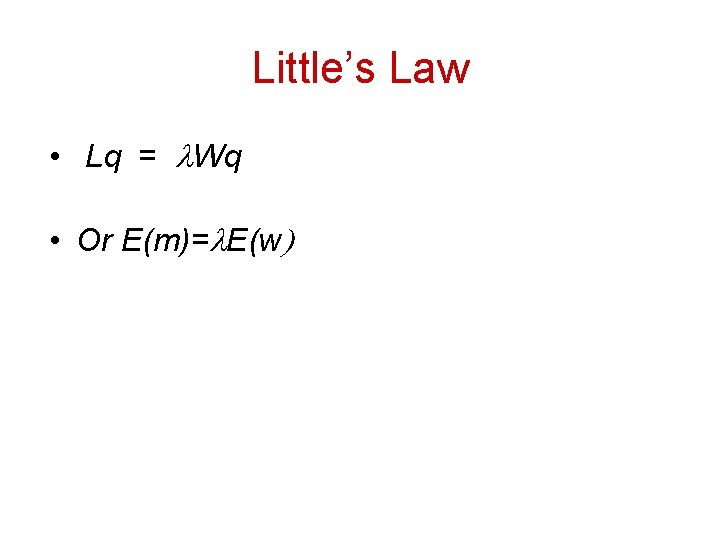
Little’s Law • Lq = l. Wq • Or E(m)=l. E(w)

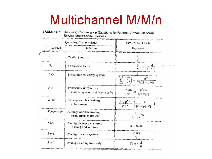
Multichannel M/M/n

M/M/1 Example • Park scenario. • Arrivals: negative exponentially distributed, arrival rate = 180 vph (3 vehs/minute) • Park ranger takes an average of 15 sec to distribute brochures. The service time distribution is also negative exponential.

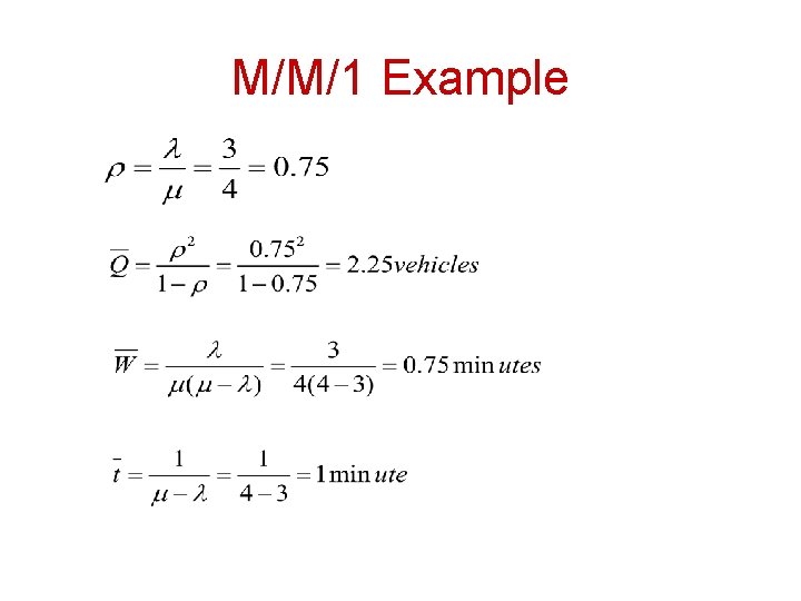
M/M/1 Example

Stochastic Queuing Example: Random Delay at Intersection Classical Queuing System Applications: • Poison Arrival, General (Arbitrary, but continuous) service times (M, G, 1) • Poisson Arrival, Erlang service times (M, Ea, 1) • Poison Arrival, Uniform service times (M, D, 1)