Queueing Theory l Specification of a Queue m

Queueing Theory l Specification of a Queue m. Source • Finite • Infinite m. Arrival Process m. Service Time Distribution m. Maximum Queueing System Capacity m. Number of Servers m. Queue Discipline

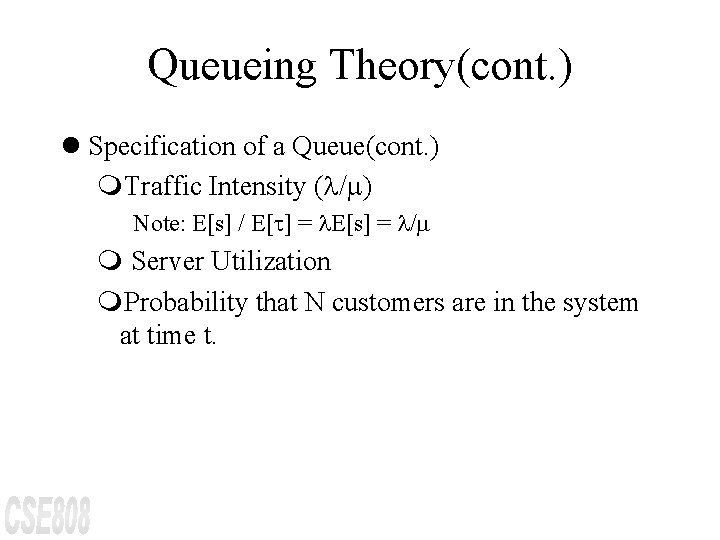
Queueing Theory(cont. ) l Specification of a Queue(cont. ) m. Traffic Intensity ( / ) Note: E[s] / E[t] = E[s] = / m Server Utilization m. Probability that N customers are in the system at time t.

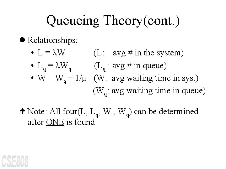
Queueing Theory(cont. ) l Relationships: s L = W (L: avg # in the system) s Lq = Wq (Lq : avg # in queue) s W = Wq + 1/ (W: avg waiting time in sys. ) (Wq: avg waiting time in queue) W Note: All four(L, Lq, W , Wq) can be determined after ONE is found

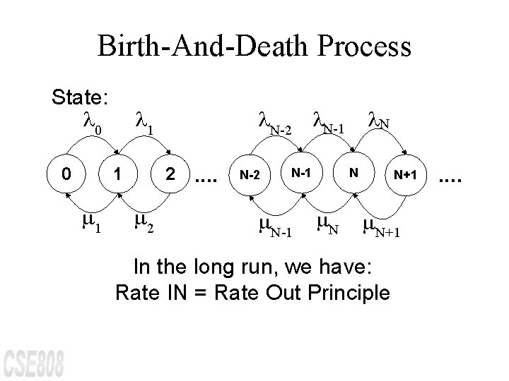
Birth-And-Death Process State: 0 0 1 1 1 N-2 N-1 2 2 . . N-2 N-1 N N+1 In the long run, we have: Rate IN = Rate Out Principle . .

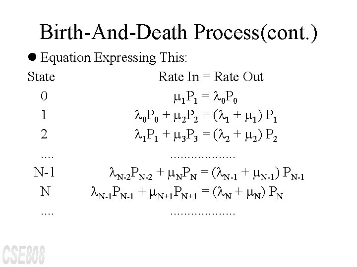
Birth-And-Death Process(cont. ) l Equation Expressing This: State Rate In = Rate Out 0 1 P 1 = 0 P 0 1 0 P 0 + 2 P 2 = ( 1 + 1) P 1 2 1 P 1 + 3 P 3 = ( 2 + 2) P 2. . . N-1 N-2 PN-2 + NPN = ( N-1 + N-1) PN-1 N N-1 PN-1 + N+1 PN+1 = ( N + N) PN. . .

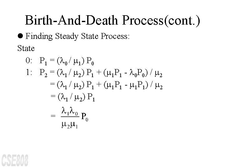
Birth-And-Death Process(cont. ) l Finding Steady State Process: State 0: P 1 = ( 0 / 1) P 0 1: P 2 = ( 1 / 2) P 1 + ( 1 P 1 - 0 P 0) / 2 = ( 1 / 2) P 1 + ( 1 P 1 - 1 P 1) / 2 = ( 1 / 2) P 1 =

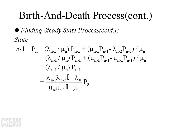
Birth-And-Death Process(cont. ) l Finding Steady State Process(cont. ): State n-1: Pn = ( n-1 / n) Pn-1 + ( n-1 Pn-1 - n-2 Pn-2) / n = ( n-1 / n) Pn-1 + ( n-1 Pn-1 - n-1 Pn-1) / n = ( n-1 / n) Pn-1

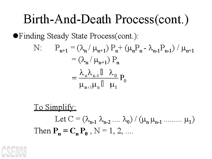
Birth-And-Death Process(cont. ) l. Finding Steady State Process(cont. ): N: Pn+1 = ( n / n+1) Pn+ ( n. Pn - n-1 Pn-1) / n+1 = ( n / n+1) Pn To Simplify: Let C = ( n-1 n-2. . 0) / ( n n-1. . 1) Then Pn = Cn P 0 , N = 1, 2, . .

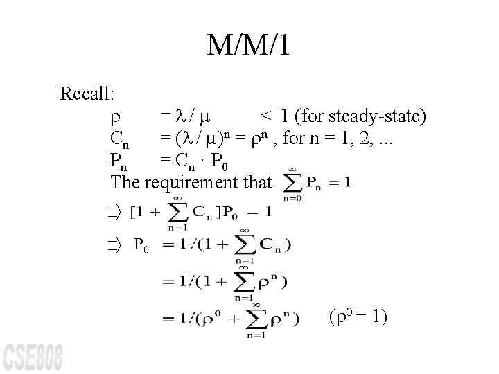
M/M/1 Recall: r = / < 1 (for steady-state) Cn = ( / )n = rn , for n = 1, 2, . . . Pn = C n · P 0 The requirement that P 0 (r 0 = 1)

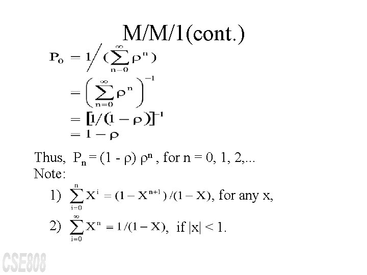
M/M/1(cont. ) Thus, Pn = (1 - r) rn , for n = 0, 1, 2, . . . Note: 1) , for any x, 2) , if |x| < 1.

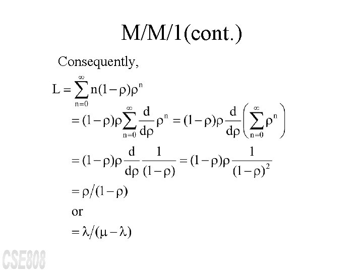
M/M/1(cont. ) Consequently,

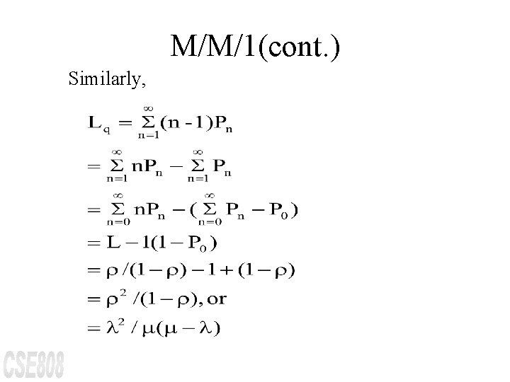
M/M/1(cont. ) Similarly,

M/M/1 Example I Traffic to a message switching center for one of the outgoing communication lines arrive in a random pattern at an average rate of 240 messages per minute. The line has a transmission rate of 800 characters per second. The message length distribution (including control characters) is approximately exponential with an average length of 176 characters. Calculate the following principal statistical measures of system performance, assuming that a very large number of message buffers are provided:

M/M/1 Example I (cont. ) l (a) Average number of messages in the system l (b) Average number of messages in the queue waiting to be transmitted. l (c) Average time a message spends in the system. l (d) Average time a message waits for transmission l (e) Probability that 10 or more messages are waiting to be transmitted. l (f) 90 th percentile waiting time in queue.

M/M/1 Example I (cont. ) l E[s] = Average Message Length / Line Speed = {176 char/message} / {800 char/sec} = 0. 22 sec/message or l = 1 / 0. 22 {message / sec} = 4. 55 message / sec l = 240 message / min = 4 message / sec l r = E[s] = / = 0. 88

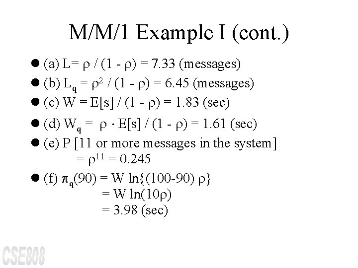
M/M/1 Example I (cont. ) l (a) L= r / (1 - r) = 7. 33 (messages) l (b) Lq = r 2 / (1 - r) = 6. 45 (messages) l (c) W = E[s] / (1 - r) = 1. 83 (sec) l (d) Wq = r E[s] / (1 - r) = 1. 61 (sec) l (e) P [11 or more messages in the system] = r 11 = 0. 245 l (f) pq(90) = W ln{(100 -90) r} = W ln(10 r) = 3. 98 (sec)

M/M/1 Example II A branch office of a large engineering firm has one on-line terminal that is connected to a central computer system during the normal eight-hour working day. Engineers, who work throughout the city, drive to the branch office to use the terminal to make routine calculations. Statistics collected over a period of time indicate that the arrival pattern of people at the branch office to use the terminal has a Poisson (random) distribution, with a mean of 10 people coming to use the terminal each day. The distribution of time spent by an engineer at a terminal is exponential, with a

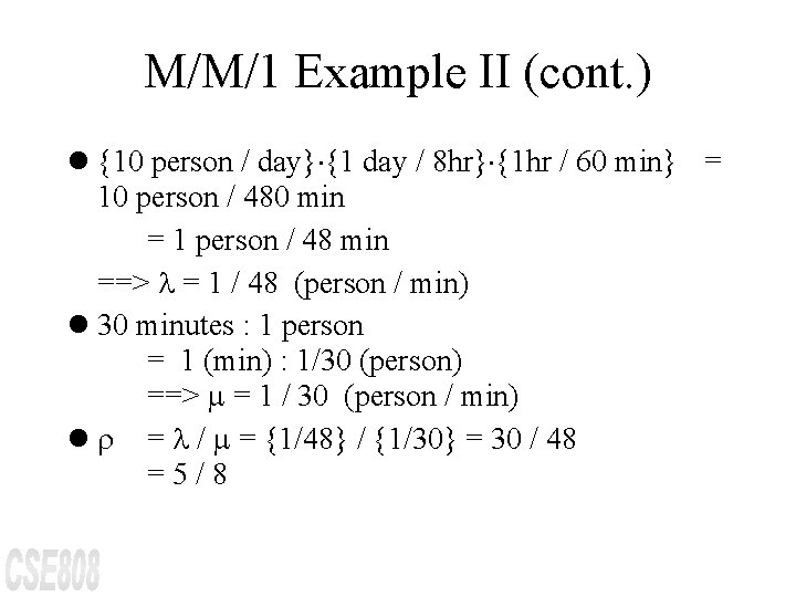
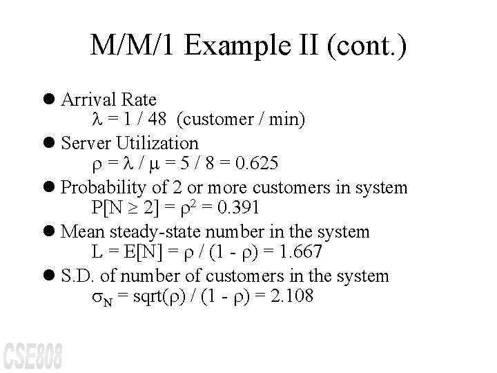
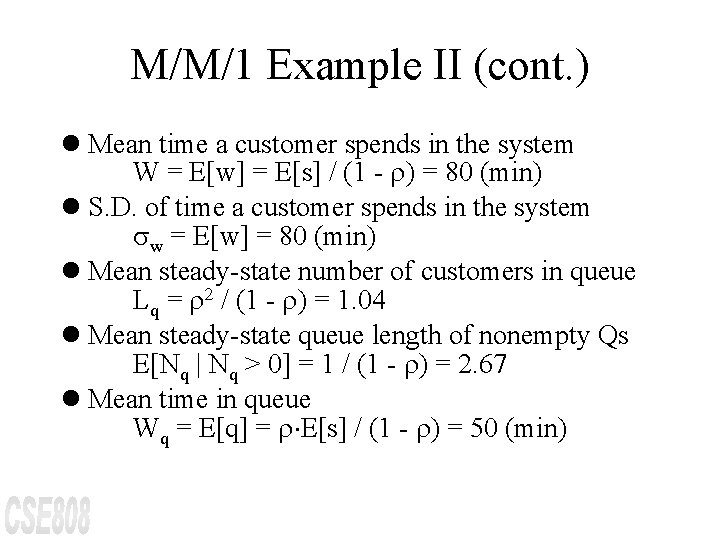
M/M/1 Example II (cont. ) mean of 30 minutes. The branch office receives complains from the staff about the terminal service. It is reported that individuals often wait over an hour to use the terminal and it rarely takes less than an hour and a half in the office to complete a few calculations. The manager is puzzled because the statistics show that the terminal is in use only 5 hours out of 8, on the average. This level of utilization would not seem to justify the acquisition of another terminal. What insight can queueing theory provide?

M/M/1 Example II (cont. ) l {10 person / day} {1 day / 8 hr} {1 hr / 60 min} = 10 person / 480 min = 1 person / 48 min ==> = 1 / 48 (person / min) l 30 minutes : 1 person = 1 (min) : 1/30 (person) ==> = 1 / 30 (person / min) l r = / = {1/48} / {1/30} = 30 / 48 =5/8

M/M/1 Example II (cont. ) l Arrival Rate = 1 / 48 (customer / min) l Server Utilization r = / = 5 / 8 = 0. 625 l Probability of 2 or more customers in system P[N ³ 2] = r 2 = 0. 391 l Mean steady-state number in the system L = E[N] = r / (1 - r) = 1. 667 l S. D. of number of customers in the system s. N = sqrt(r) / (1 - r) = 2. 108

M/M/1 Example II (cont. ) l Mean time a customer spends in the system W = E[w] = E[s] / (1 - r) = 80 (min) l S. D. of time a customer spends in the system sw = E[w] = 80 (min) l Mean steady-state number of customers in queue Lq = r 2 / (1 - r) = 1. 04 l Mean steady-state queue length of nonempty Qs E[Nq | Nq > 0] = 1 / (1 - r) = 2. 67 l Mean time in queue Wq = E[q] = r E[s] / (1 - r) = 50 (min)

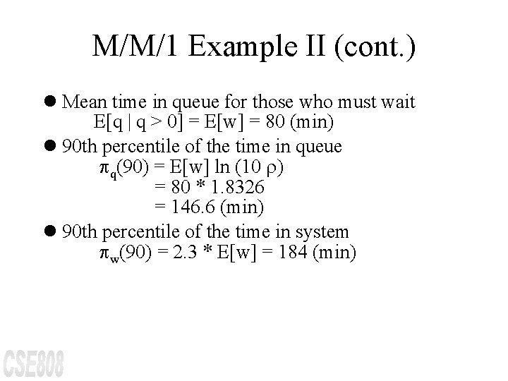
M/M/1 Example II (cont. ) l Mean time in queue for those who must wait E[q | q > 0] = E[w] = 80 (min) l 90 th percentile of the time in queue pq(90) = E[w] ln (10 r) = 80 * 1. 8326 = 146. 6 (min) l 90 th percentile of the time in system pw(90) = 2. 3 * E[w] = 184 (min)

M/M/1 Example II (cont. ) l Defined by equation P[w £ pw(90)] = 0. 9 response time of system pw(90) - amount of time in the system such that 90% of all arriving customers spend less than this amount of time in the system

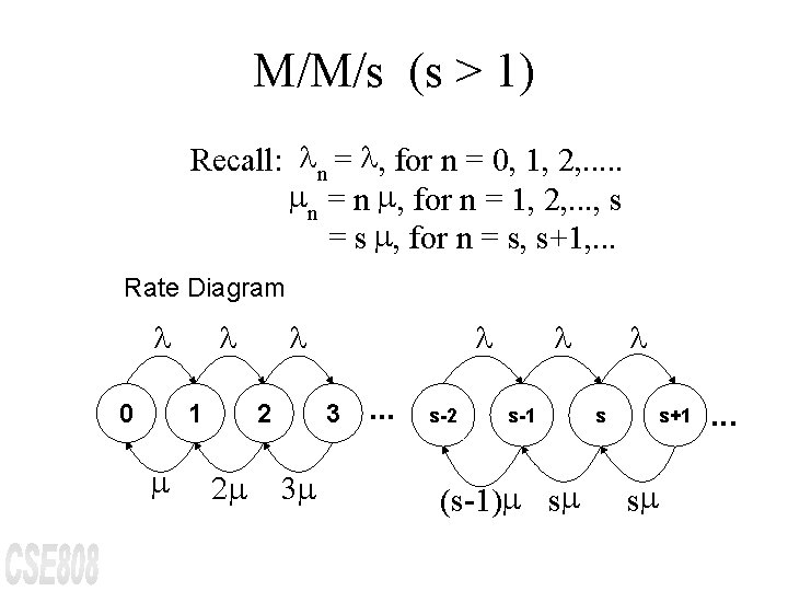
M/M/s (s > 1) Recall: n = , for n = 0, 1, 2, . . . n = n , for n = 1, 2, . . . , s = s , for n = s, s+1, . . . Rate Diagram 0 1 2 2 3 3 . . . s-2 s-1 (s-1) s s s+1 s . . .

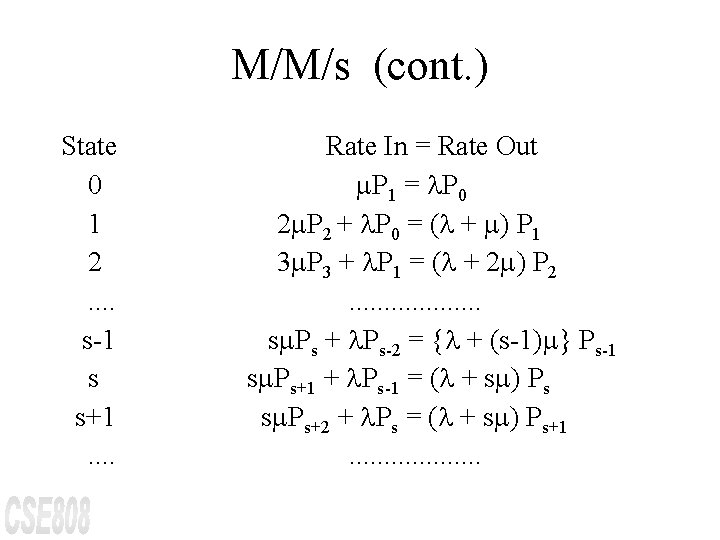
M/M/s (cont. ) State 0 1 2. . s-1 s s+1. . Rate In = Rate Out P 1 = P 0 2 P 2 + P 0 = ( + ) P 1 3 P 3 + P 1 = ( + 2 ) P 2. . . . . s Ps + Ps-2 = { + (s-1) } Ps-1 s Ps+1 + Ps-1 = ( + s ) Ps s Ps+2 + Ps = ( + s ) Ps+1. . . . .

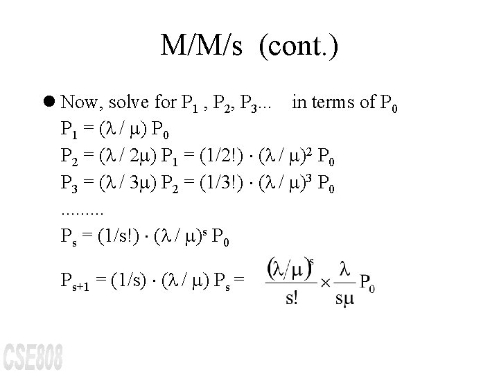
M/M/s (cont. ) l Now, solve for P 1 , P 2, P 3. . . in terms of P 0 P 1 = ( / ) P 0 P 2 = ( / 2 ) P 1 = (1/2!) ( / )2 P 0 P 3 = ( / 3 ) P 2 = (1/3!) ( / )3 P 0. . Ps = (1/s!) ( / )s P 0 Ps+1 = (1/s) ( / ) Ps =

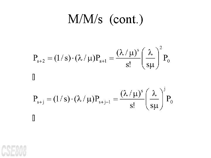
M/M/s (cont. )

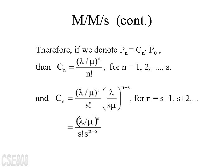
M/M/s (cont. ) Therefore, if we denote Pn = Cn P 0 , then and for n = 1, 2, . . , s. , for n = s+1, s+2, . . .

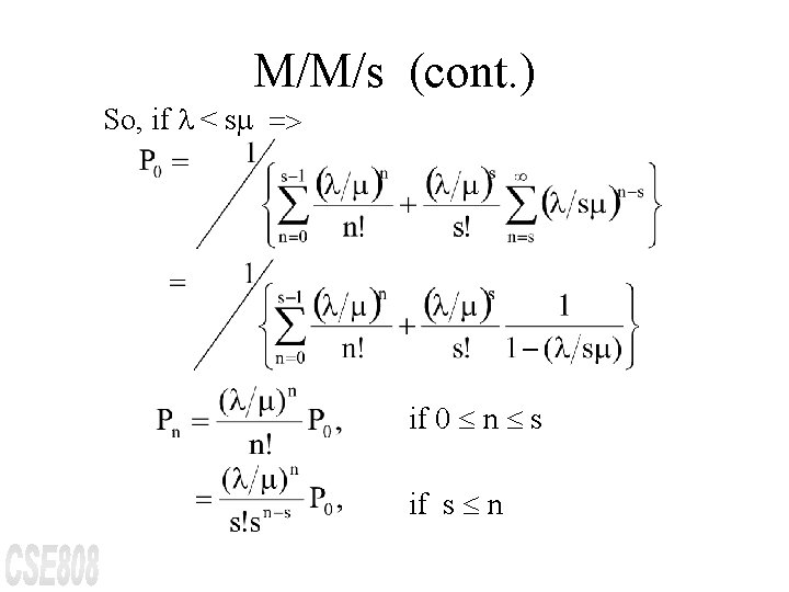
M/M/s (cont. ) So, if < s => if 0 £ n £ s if s £ n

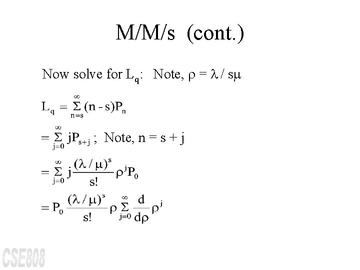
M/M/s (cont. ) Now solve for Lq: Note, r = / s ; Note, n = s + j

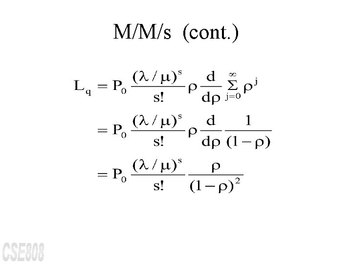
M/M/s (cont. )

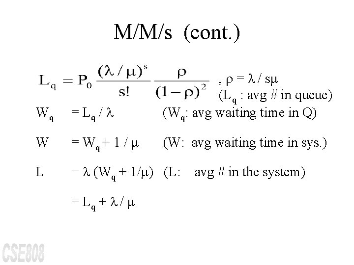
M/M/s (cont. ) Wq = Lq / , r = / s (Lq : avg # in queue) (Wq: avg waiting time in Q) W = Wq + 1 / (W: avg waiting time in sys. ) L = (Wq + 1/ ) (L: = Lq + / avg # in the system)

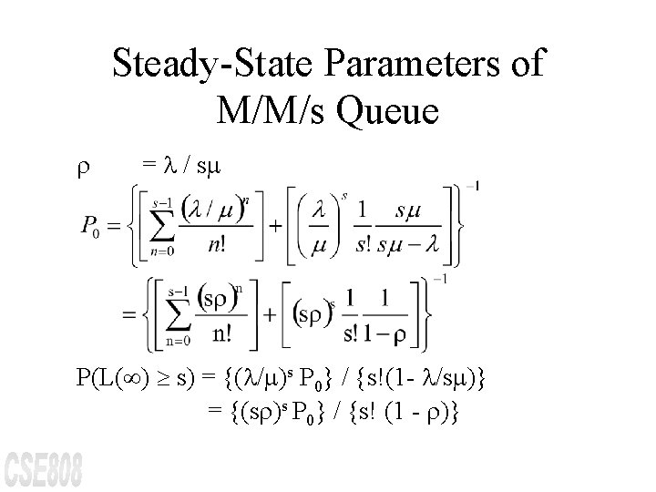
Steady-State Parameters of M/M/s Queue r = / s P(L(¥) ³ s) = {( / )s P 0} / {s!(1 - /s )} = {(sr)s P 0} / {s! (1 - r)}

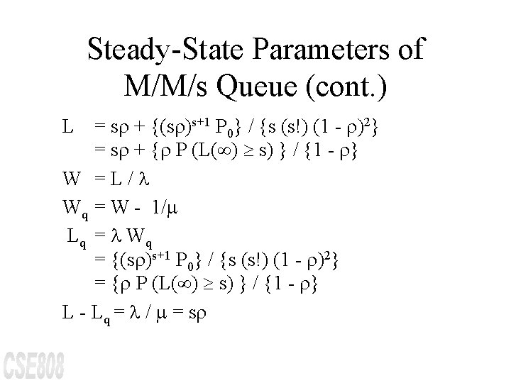
Steady-State Parameters of M/M/s Queue (cont. ) L = sr + {(sr)s+1 P 0} / {s (s!) (1 - r)2} = sr + {r P (L(¥) ³ s) } / {1 - r} W =L/ Wq = W - 1/ Lq = Wq = {(sr)s+1 P 0} / {s (s!) (1 - r)2} = {r P (L(¥) ³ s) } / {1 - r} L - Lq = / = sr

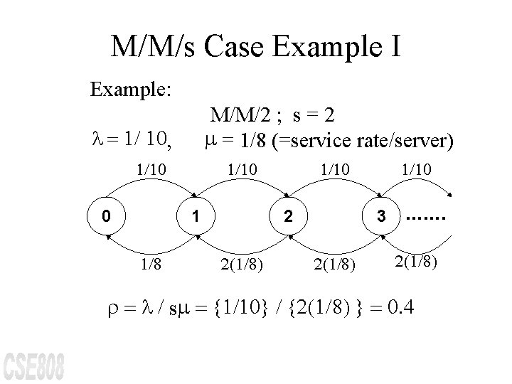
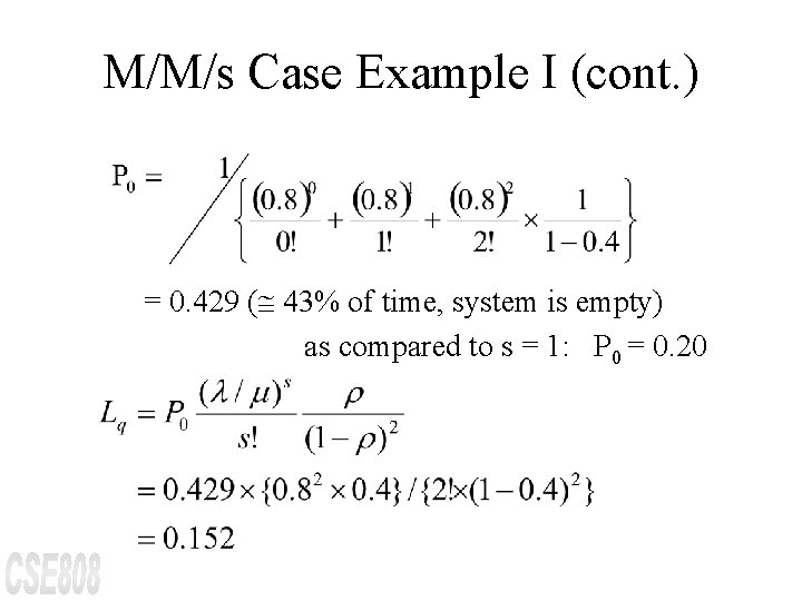
M/M/s Case Example I Example: M/M/2 ; s = 2 = 1/8 (=service rate/server) = 1/ 10, 1/10 0 1/10 1 1/8 1/10 2 2(1/8) 1/10 3 2(1/8) . . . . 2(1/8) r = / s = {1/10} / {2(1/8) } = 0. 4

M/M/s Case Example I (cont. ) = 0. 429 (@ 43% of time, system is empty) as compared to s = 1: P 0 = 0. 20

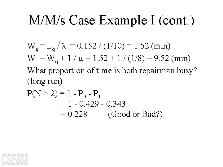
M/M/s Case Example I (cont. ) Wq = Lq / = 0. 152 / (1/10) = 1. 52 (min) W = Wq + 1 / = 1. 52 + 1 / (1/8) = 9. 52 (min) What proportion of time is both repairman busy? (long run) P(N ³ 2) = 1 - P 0 - P 1 = 1 - 0. 429 - 0. 343 = 0. 228 (Good or Bad? )

M/M/s Example II Many early examples of queueing theory applied to practical problems concerning tool cribs. Attendants manage the tool cribs while mechanics, assumed to be from an infinite calling population, arrive for service. Assume Poisson arrivals at rate 2 mechanics per minute and exponentially distributed service times with mean 40 seconds.

M/M/s Example II (cont. ) = 2 per minute, and = 60/40 = 3/2 per minute. Since, the offered load is greater than 1, that is, since, / = 2 / (3/2) = 4/3 > 1, more than one server is needed if the system is to have a statistical equilibrium. The requirement for steady state is that s > / = 4/3. Thus, at least s = 2 attendants are needed. The quantity 4/3 is the expected number of busy server, and for s ³ 2, r = 4 / (3 s) is the long-run proportion of time each server is busy. (What would happen if there were only s = 1 server? )

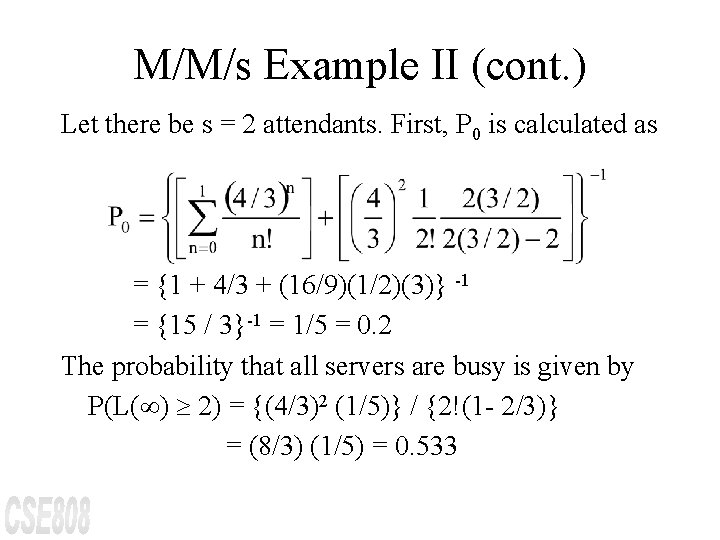
M/M/s Example II (cont. ) Let there be s = 2 attendants. First, P 0 is calculated as = {1 + 4/3 + (16/9)(1/2)(3)} -1 = {15 / 3}-1 = 1/5 = 0. 2 The probability that all servers are busy is given by P(L(¥) ³ 2) = {(4/3)2 (1/5)} / {2!(1 - 2/3)} = (8/3) (1/5) = 0. 533

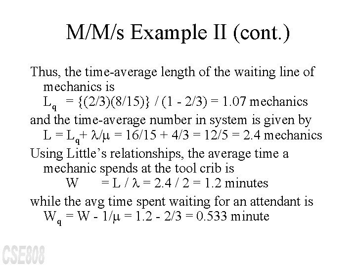
M/M/s Example II (cont. ) Thus, the time-average length of the waiting line of mechanics is Lq = {(2/3)(8/15)} / (1 - 2/3) = 1. 07 mechanics and the time-average number in system is given by L = Lq+ / = 16/15 + 4/3 = 12/5 = 2. 4 mechanics Using Little’s relationships, the average time a mechanic spends at the tool crib is W = L / = 2. 4 / 2 = 1. 2 minutes while the avg time spent waiting for an attendant is Wq = W - 1/ = 1. 2 - 2/3 = 0. 533 minute

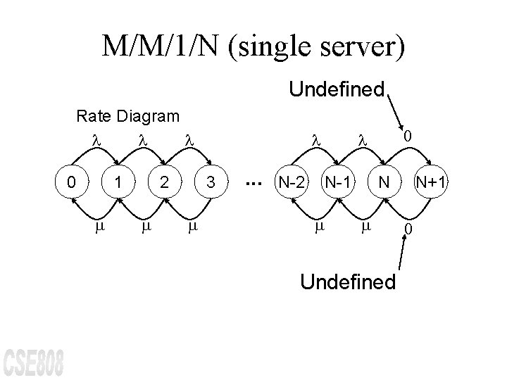
M/M/1/N (single server) Undefined Rate Diagram 0 1 2 3 . . . N-2 N-1 0 N Undefined N+1 0

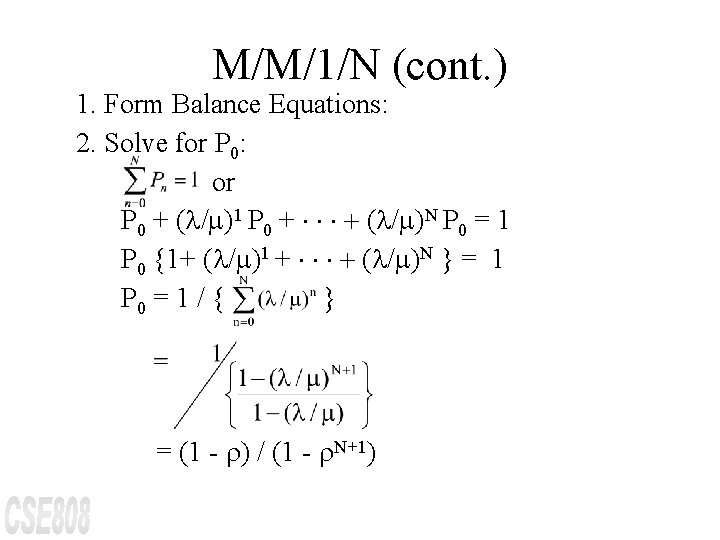
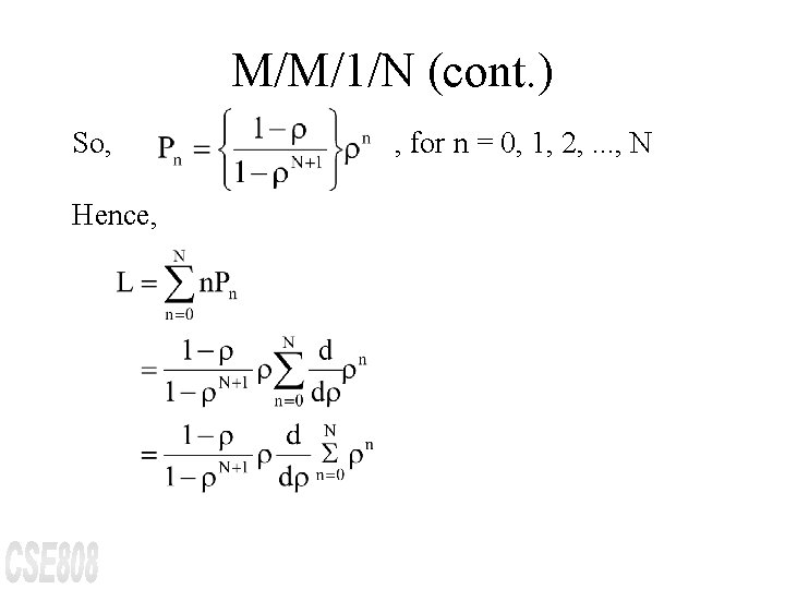
M/M/1/N (cont. ) 1. Form Balance Equations: 2. Solve for P 0: or P 0 + ( / )1 P 0 + + ( / )N P 0 = 1 P 0 {1+ ( / )1 + + ( / )N } = 1 P 0 = 1 / { } = (1 - r) / (1 - r. N+1)

M/M/1/N (cont. ) So, Hence, , for n = 0, 1, 2, . . . , N

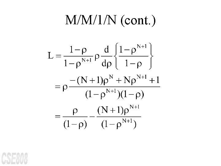
M/M/1/N (cont. )

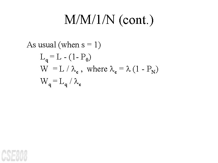
M/M/1/N (cont. ) As usual (when s = 1) Lq = L - (1 - P 0) W = L / e , where e = (1 - PN) Wq = Lq / e

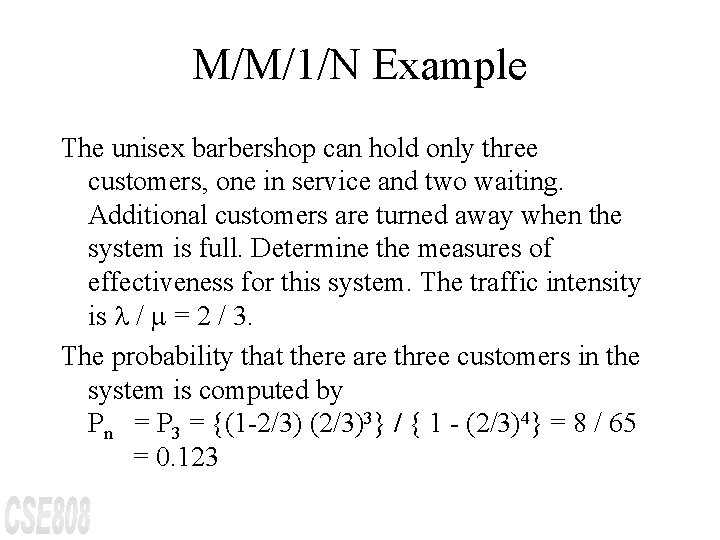
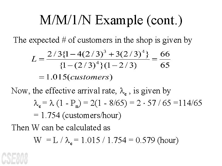
M/M/1/N Example The unisex barbershop can hold only three customers, one in service and two waiting. Additional customers are turned away when the system is full. Determine the measures of effectiveness for this system. The traffic intensity is / = 2 / 3. The probability that there are three customers in the system is computed by Pn = P 3 = {(1 -2/3) (2/3)3} / { 1 - (2/3)4} = 8 / 65 = 0. 123

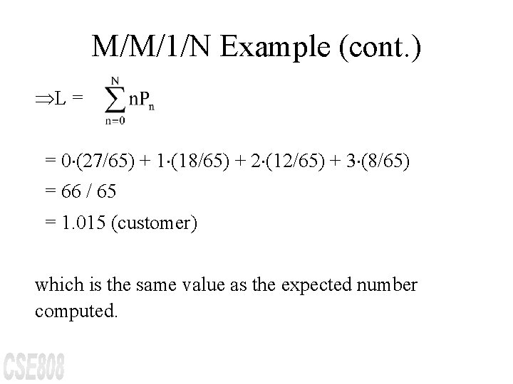
M/M/1/N Example (cont. ) The expected # of customers in the shop is given by Now, the effective arrival rate, e , is given by e = (1 - Pn) = 2(1 - 8/65) = 2 57 / 65 =114/65 = 1. 754 (customers/hour) Then W can be calculated as W = L / e = 1. 015 / 1. 754 = 0. 579 (hour)

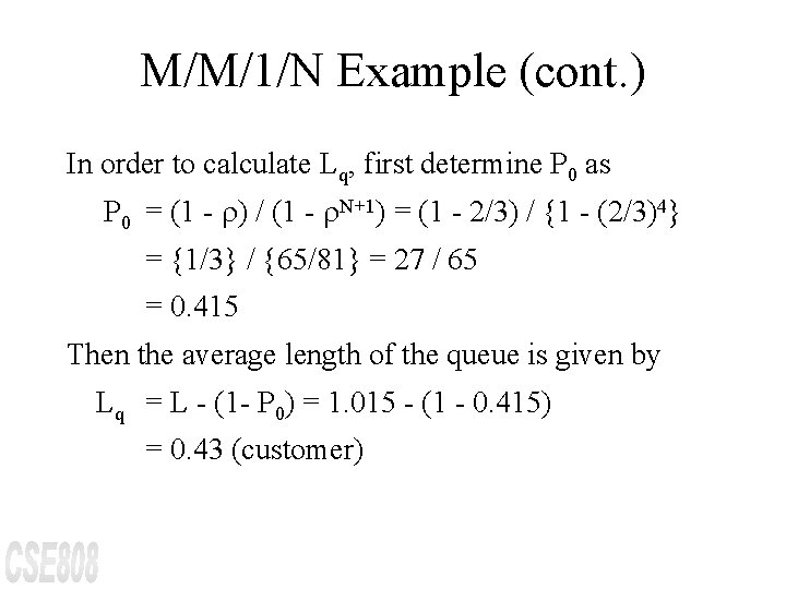
M/M/1/N Example (cont. ) In order to calculate Lq, first determine P 0 as P 0 = (1 - r) / (1 - r. N+1) = (1 - 2/3) / {1 - (2/3)4} = {1/3} / {65/81} = 27 / 65 = 0. 415 Then the average length of the queue is given by Lq = L - (1 - P 0) = 1. 015 - (1 - 0. 415) = 0. 43 (customer)

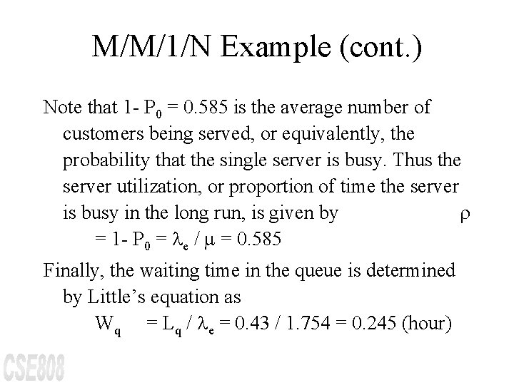
M/M/1/N Example (cont. ) Note that 1 - P 0 = 0. 585 is the average number of customers being served, or equivalently, the probability that the single server is busy. Thus the server utilization, or proportion of time the server is busy in the long run, is given by r = 1 - P 0 = e / = 0. 585 Finally, the waiting time in the queue is determined by Little’s equation as Wq = Lq / e = 0. 43 / 1. 754 = 0. 245 (hour)

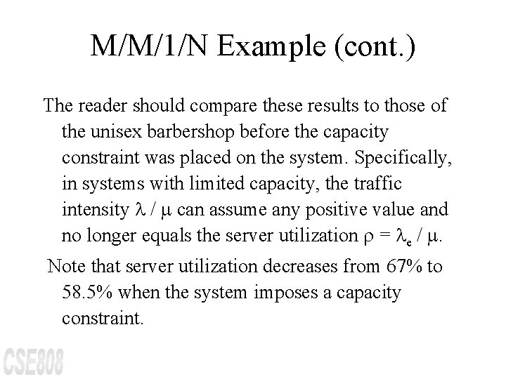
M/M/1/N Example (cont. ) The reader should compare these results to those of the unisex barbershop before the capacity constraint was placed on the system. Specifically, in systems with limited capacity, the traffic intensity / can assume any positive value and no longer equals the server utilization r = e / . Note that server utilization decreases from 67% to 58. 5% when the system imposes a capacity constraint.

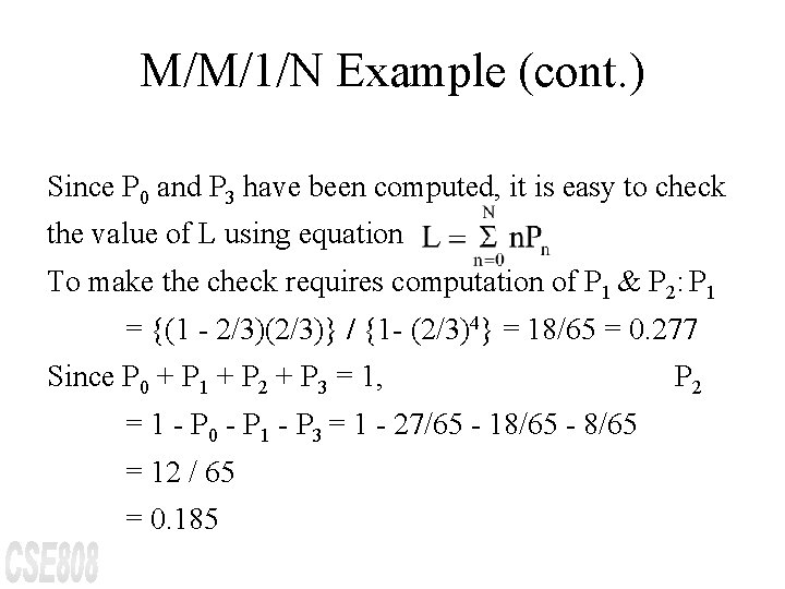
M/M/1/N Example (cont. ) Since P 0 and P 3 have been computed, it is easy to check the value of L using equation To make the check requires computation of P 1 & P 2: P 1 = {(1 - 2/3)(2/3)} / {1 - (2/3)4} = 18/65 = 0. 277 Since P 0 + P 1 + P 2 + P 3 = 1, = 1 - P 0 - P 1 - P 3 = 1 - 27/65 - 18/65 - 8/65 = 12 / 65 = 0. 185 P 2

M/M/1/N Example (cont. ) ÞL = = 0 (27/65) + 1 (18/65) + 2 (12/65) + 3 (8/65) = 66 / 65 = 1. 015 (customer) which is the same value as the expected number computed.

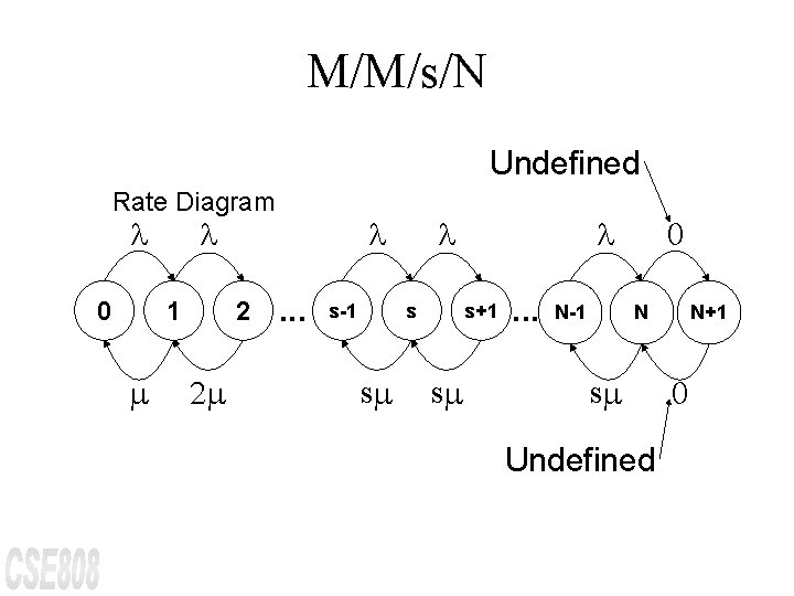
M/M/s/N Undefined Rate Diagram 0 1 2 2 . . . s-1 s s s+1 s . . . N-1 0 N s Undefined N+1 0

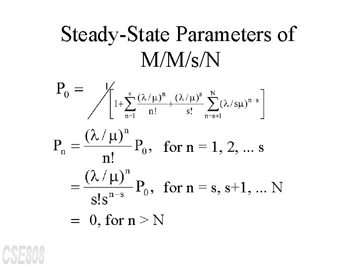
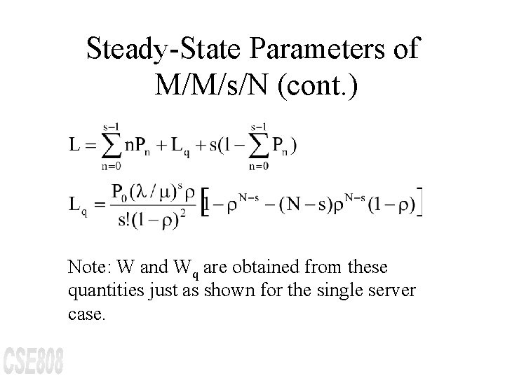
Steady-State Parameters of M/M/s/N for n = 1, 2, . . . s for n = s, s+1, . . . N 0, for n > N

Steady-State Parameters of M/M/s/N (cont. ) Note: W and Wq are obtained from these quantities just as shown for the single server case.

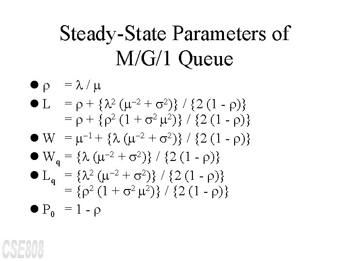
Steady-State Parameters of M/G/1 Queue lr = / l L = r + { 2 ( -2 + s 2)} / {2 (1 - r)} = r + {r 2 (1 + s 2 2)} / {2 (1 - r)} l W = -1 + { ( -2 + s 2)} / {2 (1 - r)} l Wq = { ( -2 + s 2)} / {2 (1 - r)} l Lq = { 2 ( -2 + s 2)} / {2 (1 - r)} = {r 2 (1 + s 2 2)} / {2 (1 - r)} l P 0 = 1 - r

M/G/1 Example There are two workers competing for a job. Able claims an average service time which is faster than Baker’s, but Baker claims to be more consistent, if not as fast. The arrivals occur according to a Poisson process at a rate of = 2 per hour. (1/30 per minute). Able’s statistics are an average service time of 24 minutes with a standard deviation of 20 minutes. Baker’s service statistics are an average service time of 25 minutes, but a standard deviation of only 2 minutes. If the average length of the queue is the criterion for hiring, which worker should be hired?

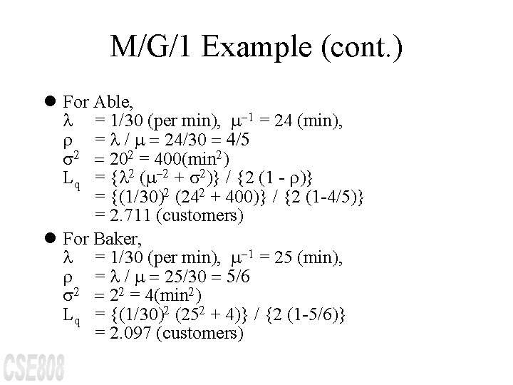
M/G/1 Example (cont. ) l For Able, = 1/30 (per min), -1 = 24 (min), r = / = 24/30 = 4/5 s 2 = 202 = 400(min 2) Lq = { 2 ( -2 + s 2)} / {2 (1 - r)} = {(1/30)2 (242 + 400)} / {2 (1 -4/5)} = 2. 711 (customers) l For Baker, = 1/30 (per min), -1 = 25 (min), r = / = 25/30 = 5/6 s 2 = 22 = 4(min 2) Lq = {(1/30)2 (252 + 4)} / {2 (1 -5/6)} = 2. 097 (customers)

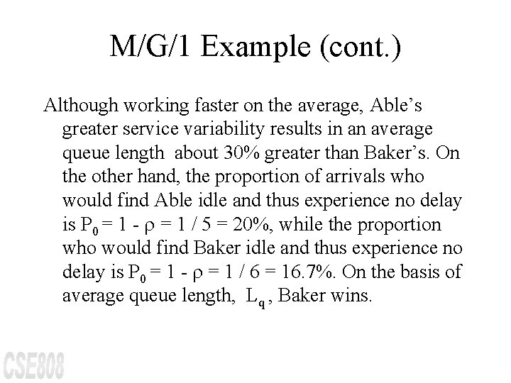
M/G/1 Example (cont. ) Although working faster on the average, Able’s greater service variability results in an average queue length about 30% greater than Baker’s. On the other hand, the proportion of arrivals who would find Able idle and thus experience no delay is P 0 = 1 - r = 1 / 5 = 20%, while the proportion who would find Baker idle and thus experience no delay is P 0 = 1 - r = 1 / 6 = 16. 7%. On the basis of average queue length, Lq , Baker wins.

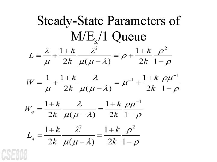
Steady-State Parameters of M/Ek/1 Queue

M/Ek/1 Example Patient arrive for a physical examination according to a Poisson process at the rate of one per hour. The physical examination requires three stages, each one independently and exponentially distributed with a service time of 15 minutes. A patient must go through all three stages before the next patient is admitted to the treatment facility. Determine the average number of delayed patients , Lq , for this system.

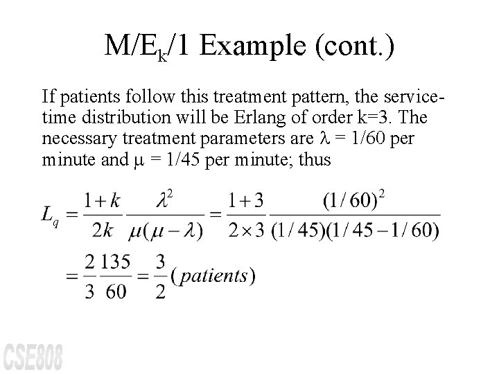
M/Ek/1 Example (cont. ) If patients follow this treatment pattern, the servicetime distribution will be Erlang of order k=3. The necessary treatment parameters are = 1/60 per minute and = 1/45 per minute; thus

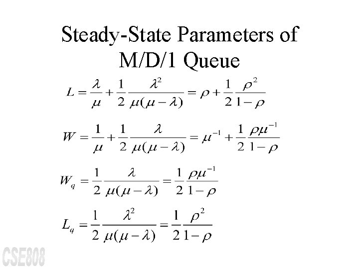
Steady-State Parameters of M/D/1 Queue

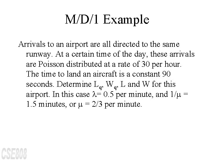
M/D/1 Example Arrivals to an airport are all directed to the same runway. At a certain time of the day, these arrivals are Poisson distributed at a rate of 30 per hour. The time to land an aircraft is a constant 90 seconds. Determine Lq, Wq, L and W for this airport. In this case = 0. 5 per minute, and 1/ = 1. 5 minutes, or = 2/3 per minute.

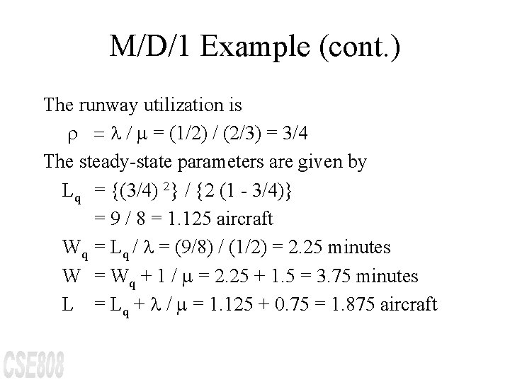
M/D/1 Example (cont. ) The runway utilization is r = / = (1/2) / (2/3) = 3/4 The steady-state parameters are given by Lq = {(3/4) 2} / {2 (1 - 3/4)} = 9 / 8 = 1. 125 aircraft Wq = Lq / = (9/8) / (1/2) = 2. 25 minutes W = Wq + 1 / = 2. 25 + 1. 5 = 3. 75 minutes L = Lq + / = 1. 125 + 0. 75 = 1. 875 aircraft

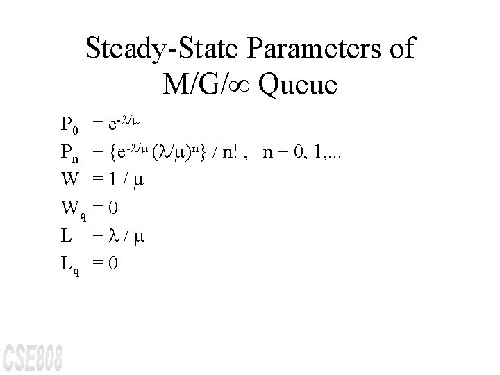
Steady-State Parameters of M/G/¥ Queue P 0 Pn W Wq L Lq = e- / = {e- / ( / )n} / n! , n = 0, 1, . . . =1/ =0 = / =0

M/G/¥ Example Prior to introducing their new on-line computer information service, The Connection must plan their system capacity in terms of the number of users that can be logged on simultaneously. If the service is successful, customers are expected to log on at a rate of = 500 per hour, according to a Poisson process, and stay connected for an average of 1/ = 20 minutes (or 1/3 hour). In the real system there will be an upper limit on simultaneous users, but for planning purpose The

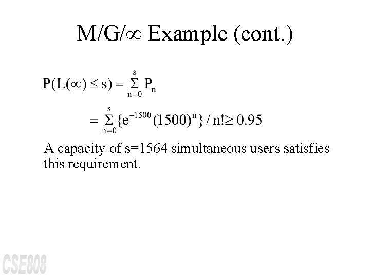
M/G/¥ Example (cont. ) Connection can pretend that the number of simultaneous users is infinite. An M/G/¥ model of the system implies that the expected number of simultaneous users is L = / = 500(3) = 1500, so a capacity greater than 1500 is certainly required. To ensure that they have adequate capacity 95% of the time, The Connection could allow the number of simultaneous users to be the smallest value s such that

M/G/¥ Example (cont. ) A capacity of s=1564 simultaneous users satisfies this requirement.

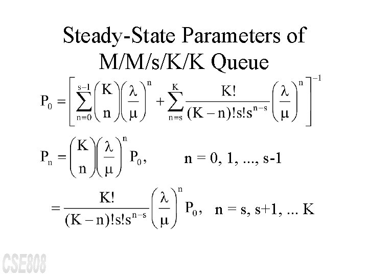
Steady-State Parameters of M/M/s/K/K Queue n = 0, 1, . . . , s-1 n = s, s+1, . . . K

Steady-State Parameters of M/M/s/K/K Queue (cont. ) W Wq r = L / e = Lq / e = (L - Lq) / s = e / s

M/M/s/K/K Example There are two workers that are responsible for 10 milling machines. The machines run on the average of 20 minutes, then require an average 5 minute service period both times exponentially distributed. Therefore, = 1/20 and = 1/5. Determine the various measures of performance for this system.

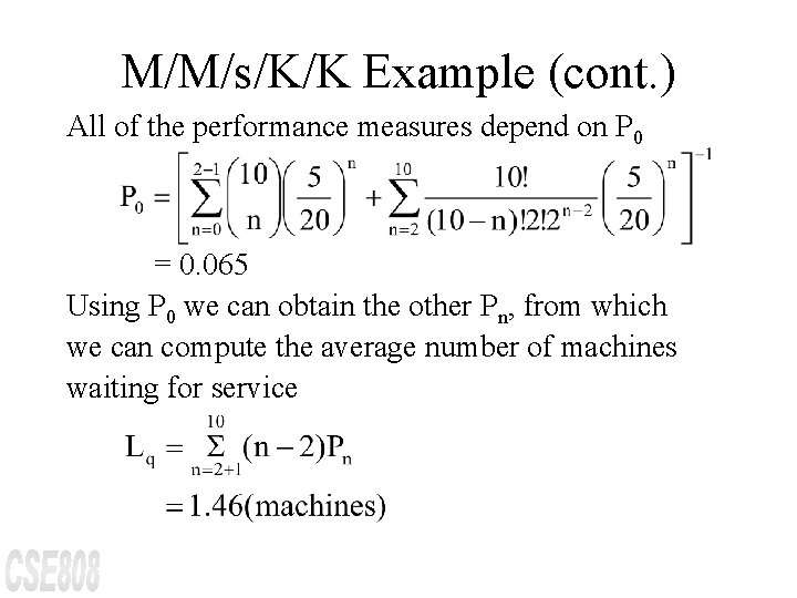
M/M/s/K/K Example (cont. ) All of the performance measures depend on P 0 = 0. 065 Using P 0 we can obtain the other Pn, from which we can compute the average number of machines waiting for service

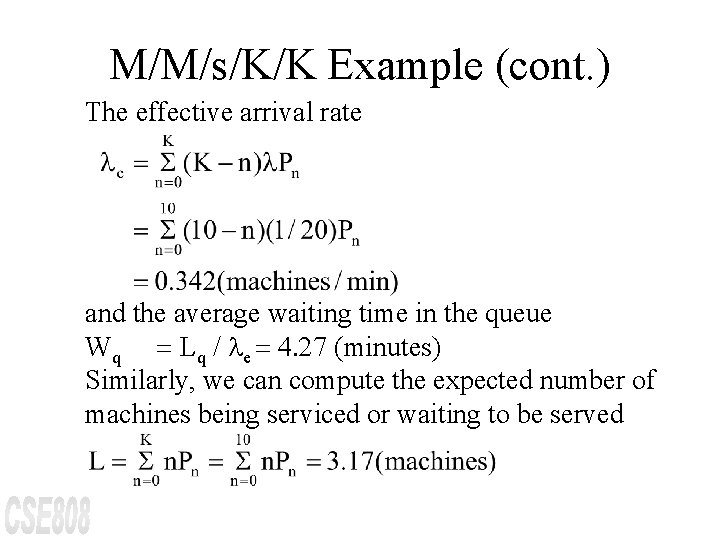
M/M/s/K/K Example (cont. ) The effective arrival rate and the average waiting time in the queue Wq = Lq / e = 4. 27 (minutes) Similarly, we can compute the expected number of machines being serviced or waiting to be served

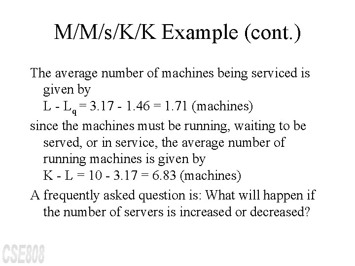
M/M/s/K/K Example (cont. ) The average number of machines being serviced is given by L - Lq = 3. 17 - 1. 46 = 1. 71 (machines) since the machines must be running, waiting to be served, or in service, the average number of running machines is given by K - L = 10 - 3. 17 = 6. 83 (machines) A frequently asked question is: What will happen if the number of servers is increased or decreased?

M/M/s/K/K Example (cont. ) If the number of workers in this example increases to three(s=3), then the time-average number of running machines increases to K - L = 7. 74 (machines) an increase of 0. 91 machine, on the average. Conversely, what happens if the number of servers decreases to one? Then the time-average number of running machines decreases to K - L = 3. 98 (machines)

M/M/s/K/K Example (cont. ) The decrease from two to one server has resulted in a drop of nearly three machines running, on the average. This example illustrates several general relationships that have been found to hold for almost all queues. If the number of servers is decreased, delays, server utilization, and the probability of an arrival having to wait to begin service all increase.