Queueing Theory I Summary n n n Littles

Queueing Theory I

Summary n n n Little’s Law Queueing System Notation Stationary Analysis of Elementary Queueing Systems ¨ M/M/1 ¨ M/M/m ¨ M/M/1/K ¨…

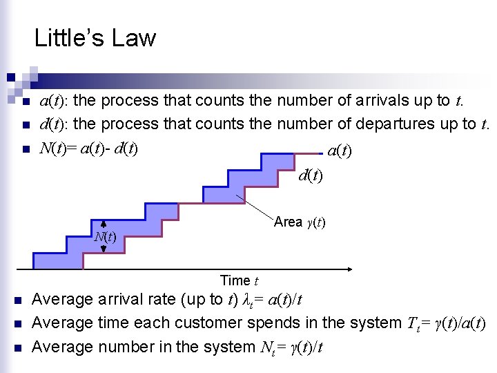
Little’s Law n n n a(t): the process that counts the number of arrivals up to t. d(t): the process that counts the number of departures up to t. N(t)= a(t)- d(t) a(t) d(t) Area γ(t) N(t) Time t n n n Average arrival rate (up to t) λt= a(t)/t Average time each customer spends in the system Tt= γ(t)/a(t) Average number in the system Nt= γ(t)/t

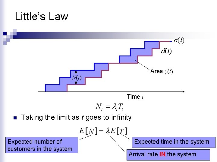
Little’s Law a(t) d(t) Area γ(t) N(t) Time t n Taking the limit as t goes to infinity Expected number of customers in the system Expected time in the system Arrival rate IN the system

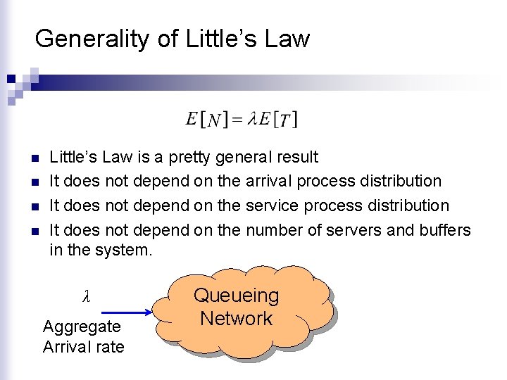
Generality of Little’s Law n n Little’s Law is a pretty general result It does not depend on the arrival process distribution It does not depend on the service process distribution It does not depend on the number of servers and buffers in the system. λ Aggregate Arrival rate Queueing Network

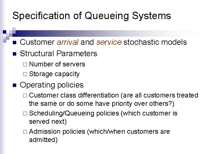
Specification of Queueing Systems n n Customer arrival and service stochastic models Structural Parameters ¨ Number of servers ¨ Storage capacity n Operating policies ¨ Customer class differentiation (are all customers treated the same or do some have priority over others? ) ¨ Scheduling/Queueing policies (which customer is served next) ¨ Admission policies (which/when customers are admitted)

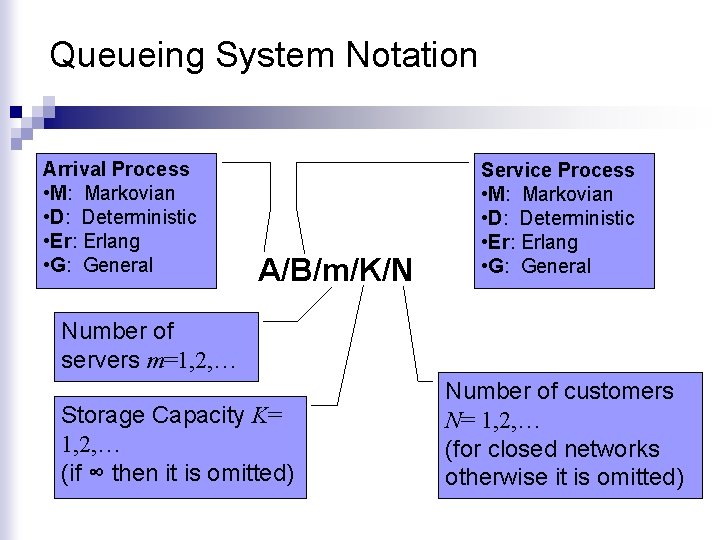
Queueing System Notation Arrival Process • M: Markovian • D: Deterministic • Er: Erlang • G: General A/B/m/K/N Service Process • M: Markovian • D: Deterministic • Er: Erlang • G: General Number of servers m=1, 2, … Storage Capacity K= 1, 2, … (if ∞ then it is omitted) Number of customers N= 1, 2, … (for closed networks otherwise it is omitted)

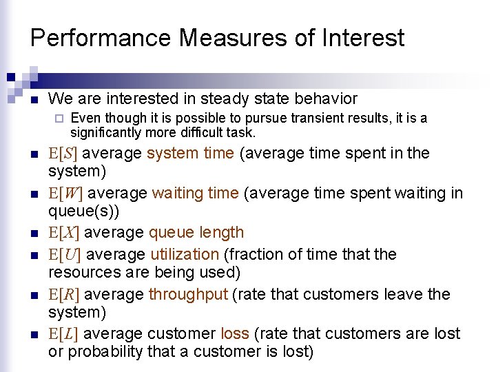
Performance Measures of Interest n We are interested in steady state behavior ¨ n n n Even though it is possible to pursue transient results, it is a significantly more difficult task. E[S] average system time (average time spent in the system) E[W] average waiting time (average time spent waiting in queue(s)) E[X] average queue length E[U] average utilization (fraction of time that the resources are being used) E[R] average throughput (rate that customers leave the system) E[L] average customer loss (rate that customers are lost or probability that a customer is lost)

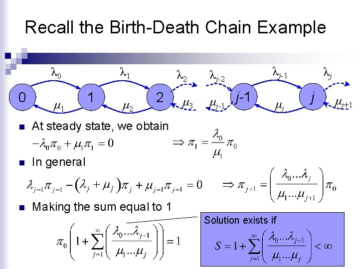
Recall the Birth-Death Chain Example λ 0 0 μ 1 λ 1 1 μ 2 λ 2 2 n At steady state, we obtain n In general n Making the sum equal to 1 μ 3 λj-2 λj-1 μj-1 μj Solution exists if λj j μj+1

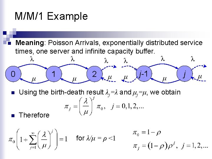
M/M/1 Example n Meaning: Poisson Arrivals, exponentially distributed service times, one server and infinite capacity buffer. λ λ λ 0 μ 1 μ 2 μ μ j-1 μ n Using the birth-death result λj=λ and μj=μ, we obtain n Therefore for λ/μ = ρ <1 j μ

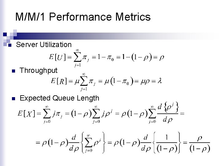
M/M/1 Performance Metrics n Server Utilization n Throughput n Expected Queue Length

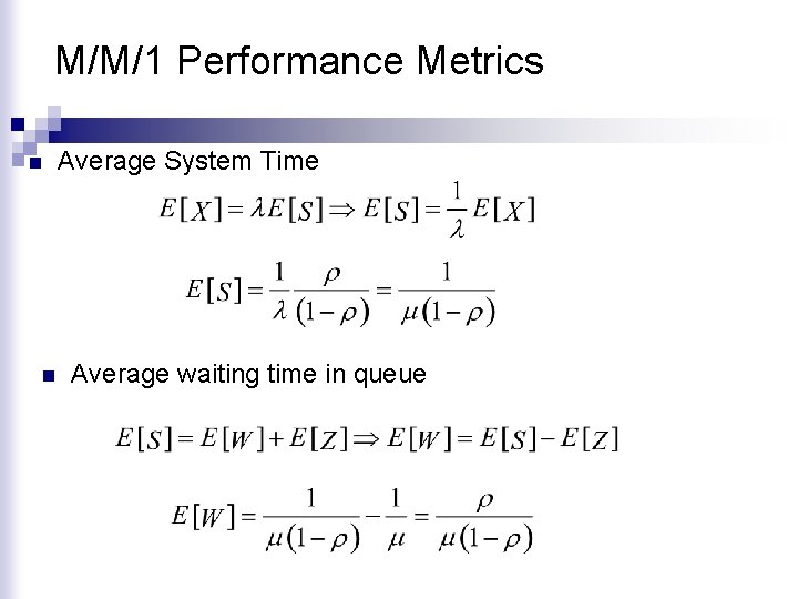
M/M/1 Performance Metrics n n Average System Time Average waiting time in queue

M/M/1 Performance Metrics Examples n μ=0. 5 Ε[S] Ε[W] Ε[Χ]

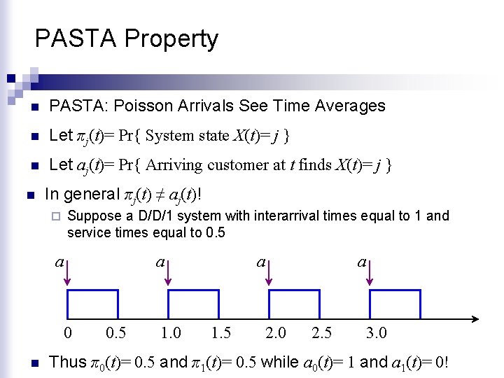
PASTA Property n PASTA: Poisson Arrivals See Time Averages n Let πj(t)= Pr{ System state X(t)= j } n Let aj(t)= Pr{ Arriving customer at t finds X(t)= j } n In general πj(t) ≠ aj(t)! Suppose a D/D/1 system with interarrival times equal to 1 and service times equal to 0. 5 ¨ a a 0 n 0. 5 1. 0 a 1. 5 a 2. 0 2. 5 3. 0 Thus π0(t)= 0. 5 and π1(t)= 0. 5 while a 0(t)= 1 and a 1(t)= 0!

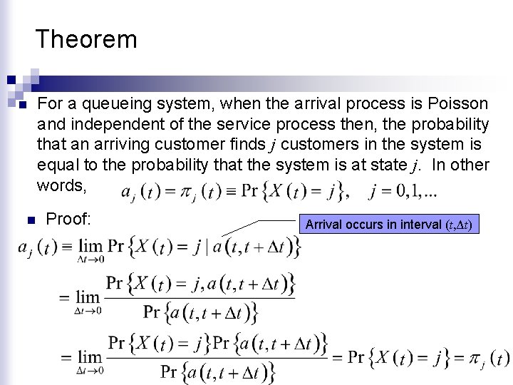
Theorem n n For a queueing system, when the arrival process is Poisson and independent of the service process then, the probability that an arriving customer finds j customers in the system is equal to the probability that the system is at state j. In other words, Proof: Arrival occurs in interval (t, Δt)

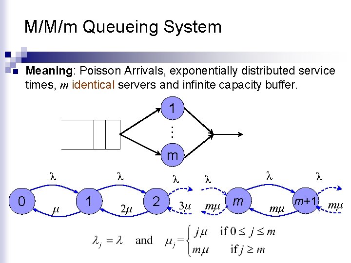
M/M/m Queueing System n Meaning: Poisson Arrivals, exponentially distributed service times, m identical servers and infinite capacity buffer. 1 … m λ 0 μ λ 1 2μ λ 2 λ λ 3μ mμ m mμ λ m+1 mμ

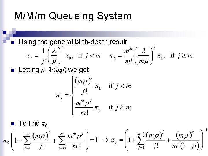
M/M/m Queueing System n Using the general birth-death result n Letting ρ=λ/(mμ) we get n To find π0

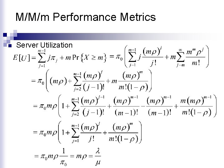
M/M/m Performance Metrics n Server Utilization

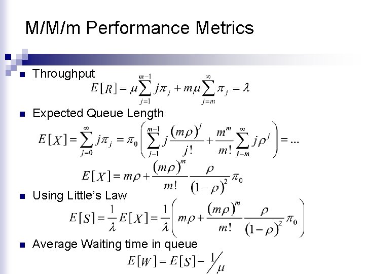
M/M/m Performance Metrics n Throughput n Expected Queue Length n Using Little’s Law n Average Waiting time in queue

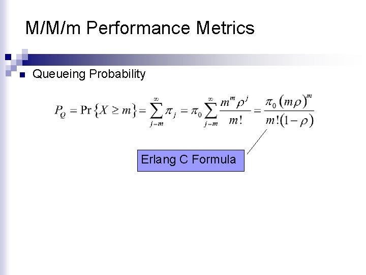
M/M/m Performance Metrics n Queueing Probability Erlang C Formula

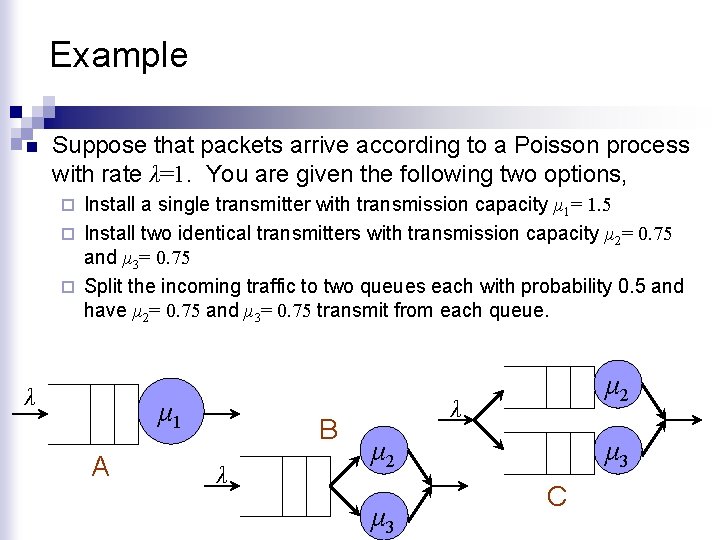
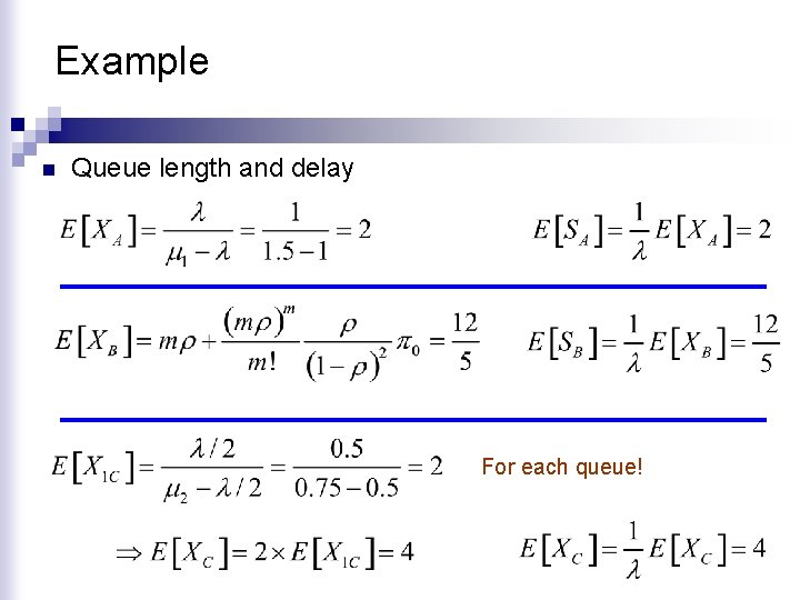
Example n Suppose that packets arrive according to a Poisson process with rate λ=1. You are given the following two options, Install a single transmitter with transmission capacity μ 1= 1. 5 ¨ Install two identical transmitters with transmission capacity μ 2= 0. 75 and μ 3= 0. 75 ¨ Split the incoming traffic to two queues each with probability 0. 5 and have μ 2= 0. 75 and μ 3= 0. 75 transmit from each queue. ¨ λ μ 1 Α Β λ μ 2 μ 3 C

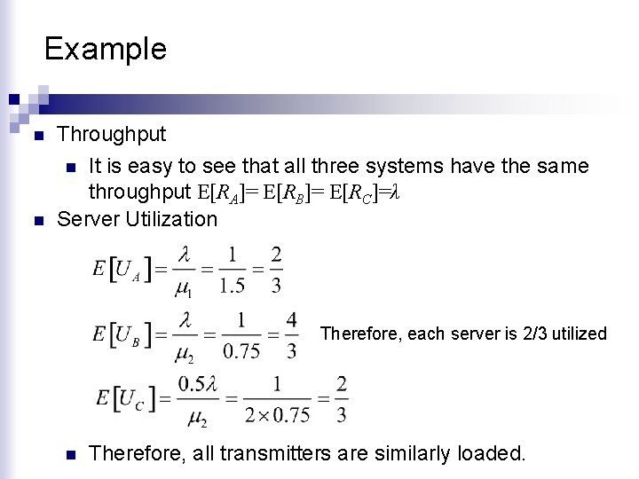
Example n n Throughput n It is easy to see that all three systems have the same throughput E[RA]= E[RB]= E[RC]=λ Server Utilization Therefore, each server is 2/3 utilized n Therefore, all transmitters are similarly loaded.

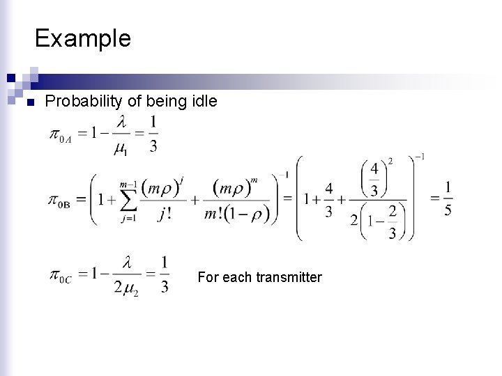
Example n Probability of being idle For each transmitter

Example n Queue length and delay For each queue!

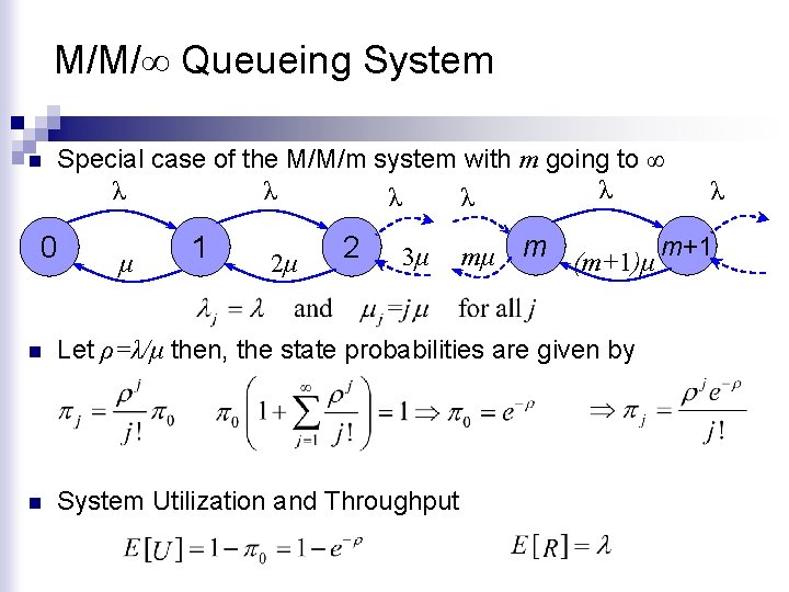
M/M/∞ Queueing System n Special case of the M/M/m system with m going to ∞ λ λ λ 0 μ 1 2μ 2 3μ mμ λ m (m+1)μ m+1 n Let ρ=λ/μ then, the state probabilities are given by n System Utilization and Throughput

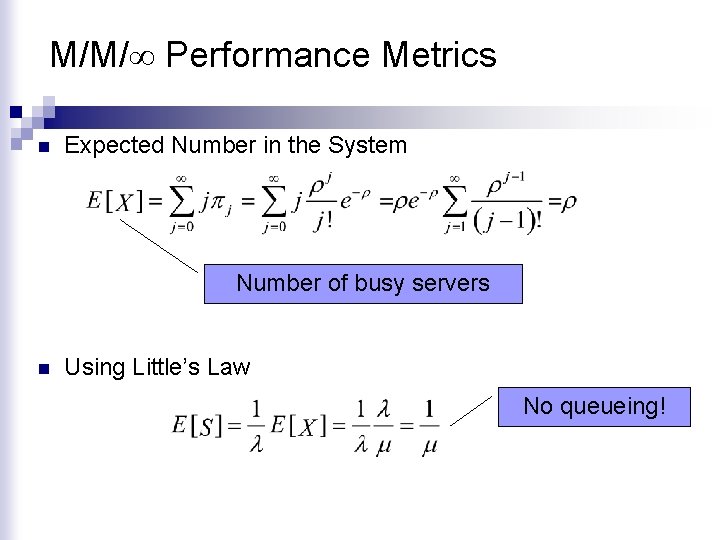
M/M/∞ Performance Metrics n Expected Number in the System Number of busy servers n Using Little’s Law No queueing!

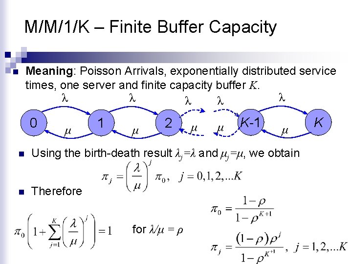
M/M/1/K – Finite Buffer Capacity n Meaning: Poisson Arrivals, exponentially distributed service times, one server and finite capacity buffer K. λ λ λ 0 μ 1 μ 2 μ μ K-1 μ n Using the birth-death result λj=λ and μj=μ, we obtain n Therefore for λ/μ = ρ K

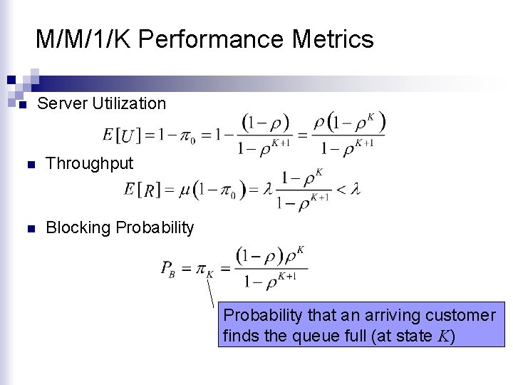
M/M/1/K Performance Metrics n Server Utilization n Throughput n Blocking Probability that an arriving customer finds the queue full (at state K)

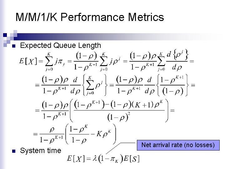
M/M/1/K Performance Metrics n n Expected Queue Length System time Net arrival rate (no losses)

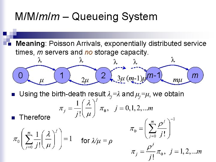
M/M/m/m – Queueing System n Meaning: Poisson Arrivals, exponentially distributed service times, m servers and no storage capacity. λ λ λ 0 μ 1 2μ 2 3μ (m-1)μ m-1 mμ n Using the birth-death result λj=λ and μj=μ, we obtain n Therefore for λ/μ = ρ m

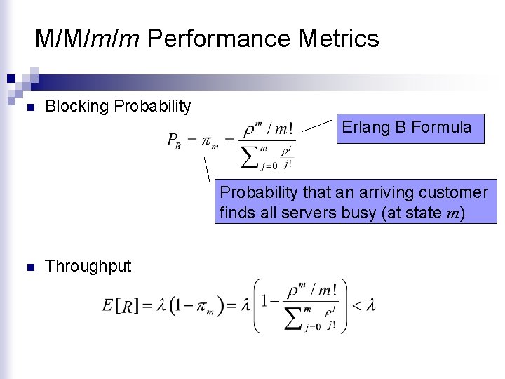
M/M/m/m Performance Metrics n Blocking Probability Erlang B Formula Probability that an arriving customer finds all servers busy (at state m) n Throughput

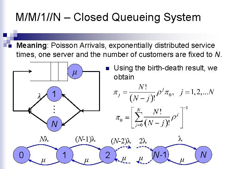
M/M/1//N – Closed Queueing System n Meaning: Poisson Arrivals, exponentially distributed service times, one server and the number of customers are fixed to N. n μ Using the birth-death result, we obtain 1 λ … N Nλ 0 μ (N-1)λ 1 μ (N-2)λ 2 μ λ 2λ μ N-1 μ N

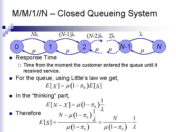
M/M/1//N – Closed Queueing System Nλ 0 n (N-1)λ 1 μ Response Time ¨ μ (N-2)λ 2 μ λ 2λ μ N-1 μ N Time from the moment the customer entered the queue until it received service. n For the queue, using Little’s law we get, n In the “thinking” part, n Therefore