Queueing System I Introduction The ultimate goal is

Queueing System I

Introduction • The ultimate goal is to achieve an economic balance between the cost of service and the cost associated with the waiting for that service. • Example—Doctor Requirement in a Emergence Room • Consider assigning an extra doctor to the emergency room, which has one doctor already. • How much can we reduce the average waiting time for patients if the extra doctor is hired?

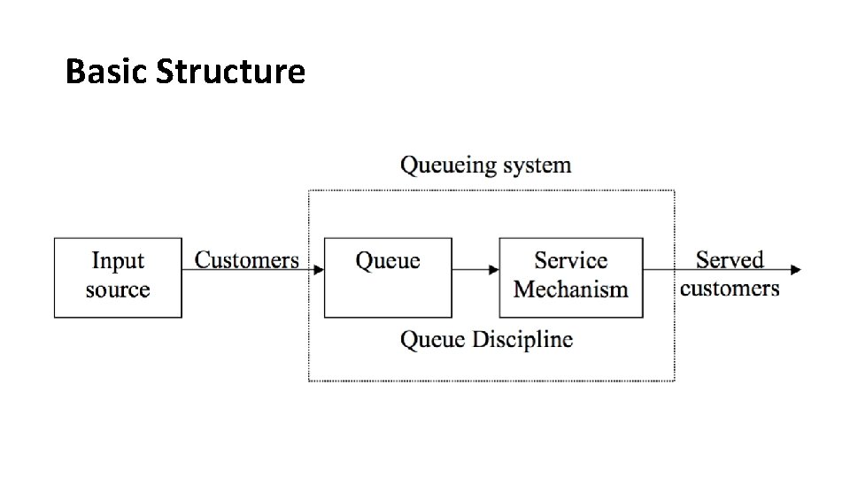
Basic Structure

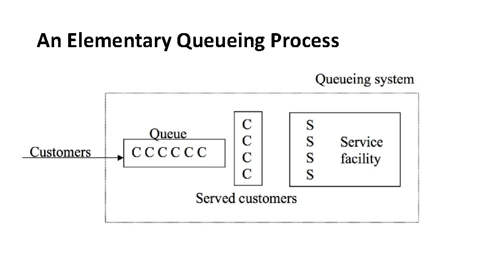
An Elementary Queueing Process

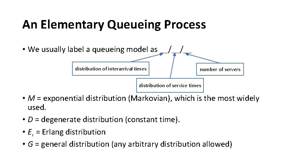
An Elementary Queueing Process • We usually label a queueing model as ＿/＿/＿ distribution of interarrival times number of servers distribution of service times • M = exponential distribution (Markovian), which is the most widely used. • D = degenerate distribution (constant time). • Er = Erlang distribution • G = general distribution (any arbitrary distribution allowed)

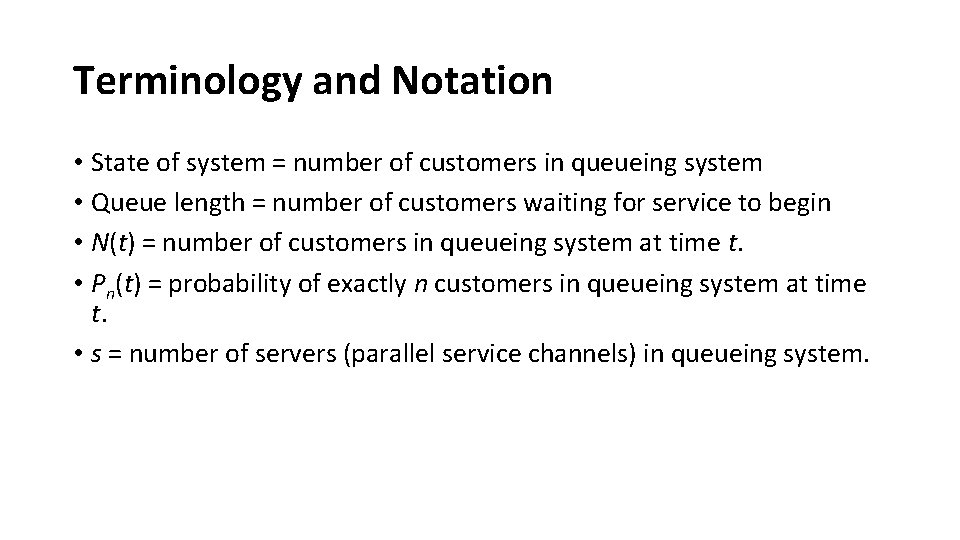
Terminology and Notation • State of system = number of customers in queueing system • Queue length = number of customers waiting for service to begin • N(t) = number of customers in queueing system at time t. • Pn(t) = probability of exactly n customers in queueing system at time t. • s = number of servers (parallel service channels) in queueing system.

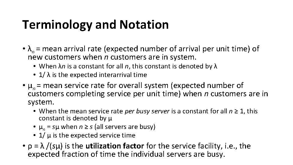
Terminology and Notation • λn = mean arrival rate (expected number of arrival per unit time) of new customers when n customers are in system. • When λn is a constant for all n, this constant is denoted by λ • 1/ λ is the expected interarrival time • μn = mean service rate for overall system (expected number of customers completing service per unit time) when n customers are in system. • When the mean service rate per busy server is a constant for all n ≥ 1, this constant is denoted by μ • μn = sμ when n ≥ s (all servers are busy) • 1/ μ is the expected service time • ρ = λ /(sμ) is the utilization factor for the service facility, i. e. , the expected fraction of time the individual servers are busy.

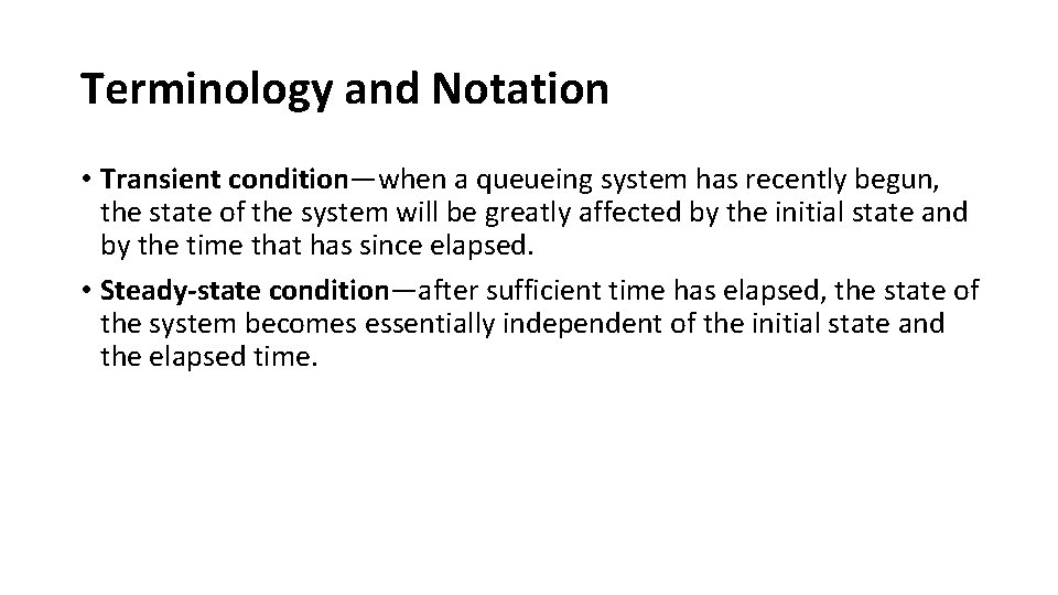
Terminology and Notation • Transient condition—when a queueing system has recently begun, the state of the system will be greatly affected by the initial state and by the time that has since elapsed. • Steady-state condition—after sufficient time has elapsed, the state of the system becomes essentially independent of the initial state and the elapsed time.

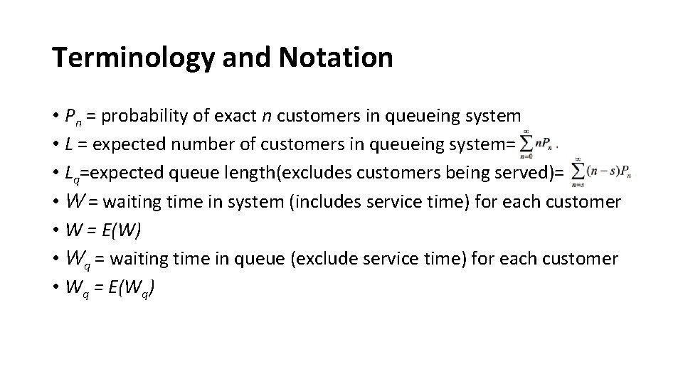
Terminology and Notation • Pn = probability of exact n customers in queueing system • L = expected number of customers in queueing system= • Lq=expected queue length(excludes customers being served)= • W = waiting time in system (includes service time) for each customer • W = E(W) • Wq = waiting time in queue (exclude service time) for each customer • Wq = E(Wq)

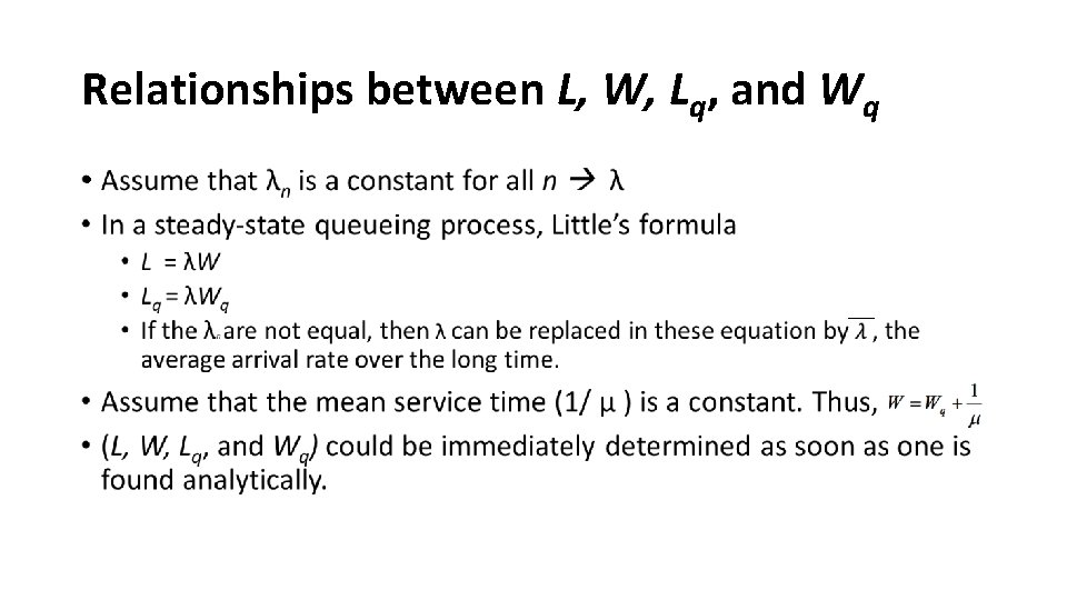
Relationships between L, W, Lq, and Wq •

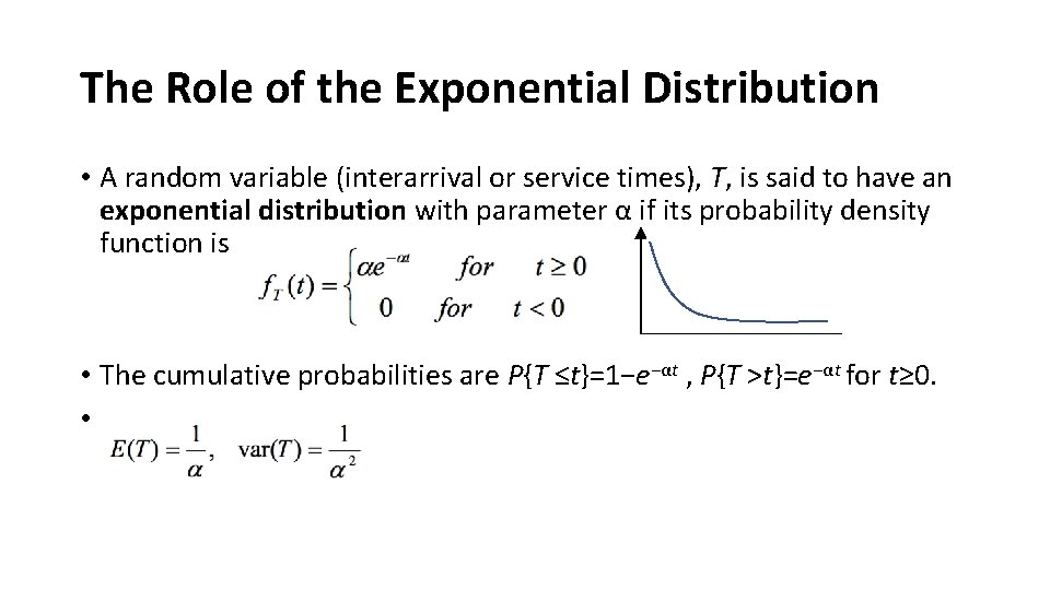
The Role of the Exponential Distribution • A random variable (interarrival or service times), T, is said to have an exponential distribution with parameter α if its probability density function is • The cumulative probabilities are P{T ≤t}=1−e−αt , P{T >t}=e−αt for t≥ 0. •

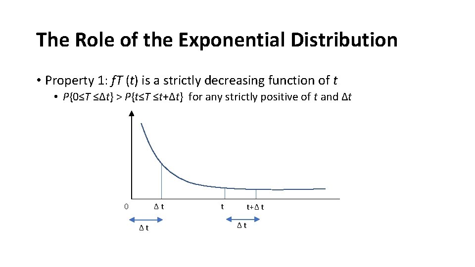
The Role of the Exponential Distribution • Property 1: f. T (t) is a strictly decreasing function of t • P{0≤T ≤Δt} > P{t≤T ≤t+Δt} for any strictly positive of t and Δt 0 Δt Δt t t+Δ t Δt

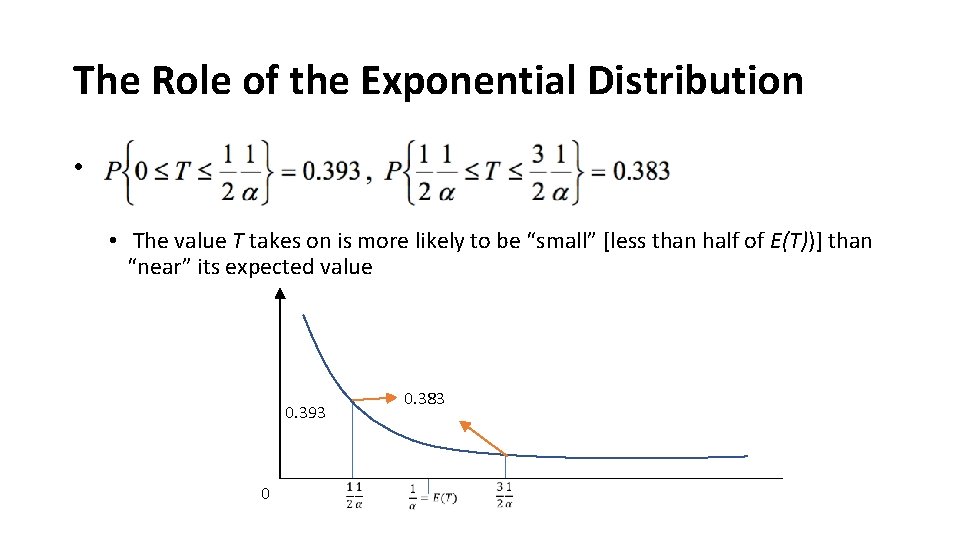
The Role of the Exponential Distribution • • The value T takes on is more likely to be “small” [less than half of E(T))] than “near” its expected value 0. 393 0 0. 383

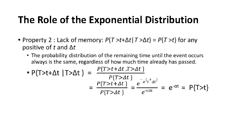
The Role of the Exponential Distribution •

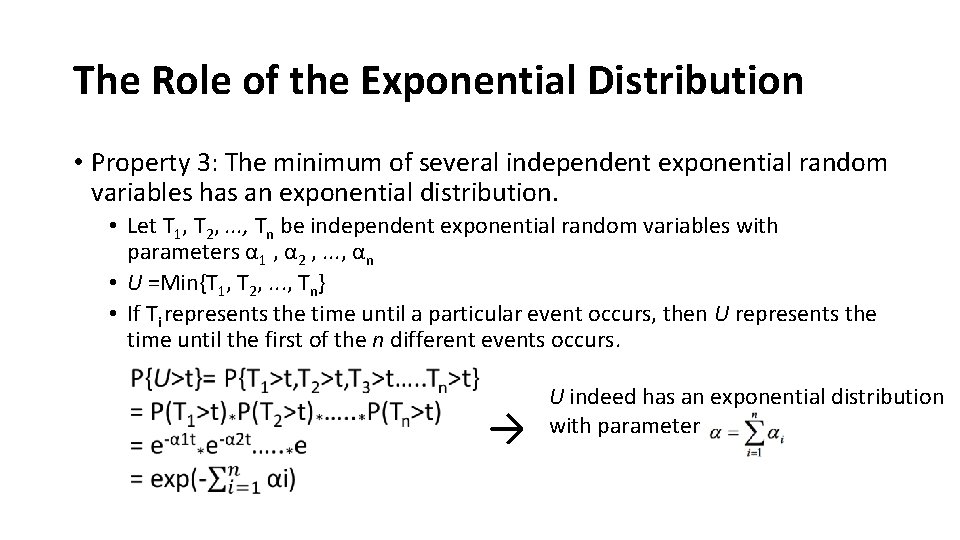
The Role of the Exponential Distribution • Property 3: The minimum of several independent exponential random variables has an exponential distribution. • Let T 1, T 2, . . . , Tn be independent exponential random variables with parameters α 1 , α 2 , . . . , αn • U =Min{T 1, T 2, . . . , Tn} • If Ti represents the time until a particular event occurs, then U represents the time until the first of the n different events occurs. → U indeed has an exponential distribution with parameter

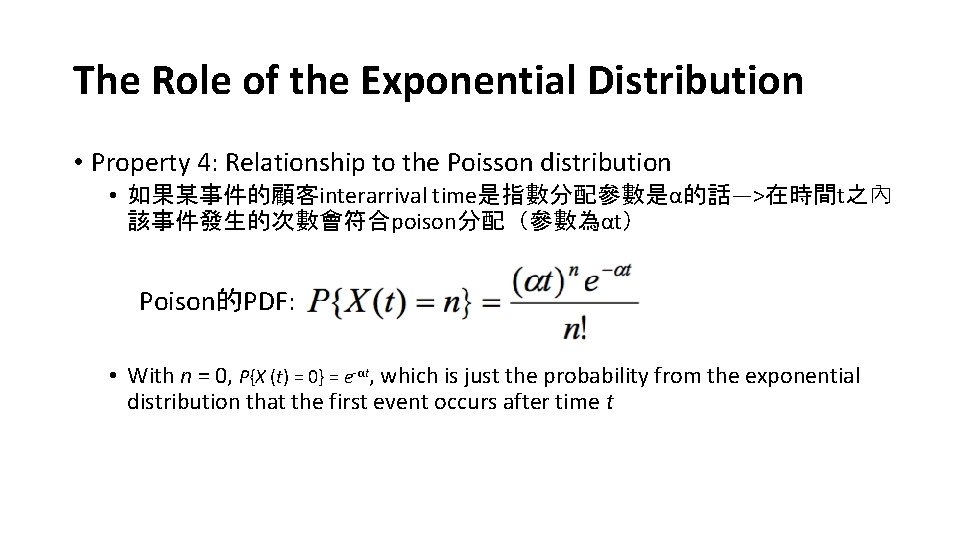
The Role of the Exponential Distribution • Property 4: Relationship to the Poisson distribution • 如果某事件的顧客interarrival time是指數分配參數是α的話—>在時間t之內 該事件發生的次數會符合poison分配（參數為αt） Poison的PDF: • With n = 0, P{X (t) = 0} = e-αt, which is just the probability from the exponential distribution that the first event occurs after time t

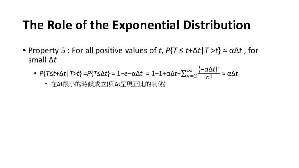
The Role of the Exponential Distribution •

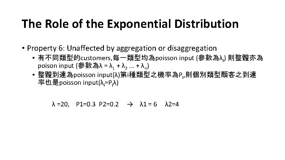
The Role of the Exponential Distribution • Property 6: Unaffected by aggregation or disaggregation • 有不同類型的customers, 每一類型均為poisson input (參數為λi) 則整體亦為 poison input (參數為λ = λ 1 + λ 2. . . + λn) • 整體到達為poisson input(λ)第i種類型之機率為Pi, 則個別類型顧客之到達 率也是poisson input(λi=Piλ) λ =20, P 1=0. 3 P 2=0. 2 → λ 1 = 6 λ 2=4