Query Processing Part 3 BTrees 1 Dense and

Query Processing Part 3: B+Trees 1

Dense and Sparse Indexes Advantage: - Simple - Index is sequential file good for scans Disadvantage: - Insertions expensive, and/or - Lose sequentiality & balance 2

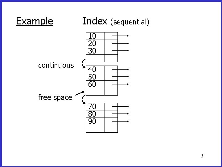
Example Index (sequential) 10 20 30 continuous 40 50 60 free space 70 80 90 3

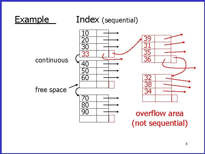
Example continuous Index 10 20 30 33 40 50 60 free space 70 80 90 (sequential) 39 31 35 36 32 38 34 overflow area (not sequential) 4

B+Trees: Main Idea • Give up on sequentiality of index • Try to get “balance” • A node corresponds to a block – Because have to read (at least) one block • Control the height by requiring nodes to be at least half full 5

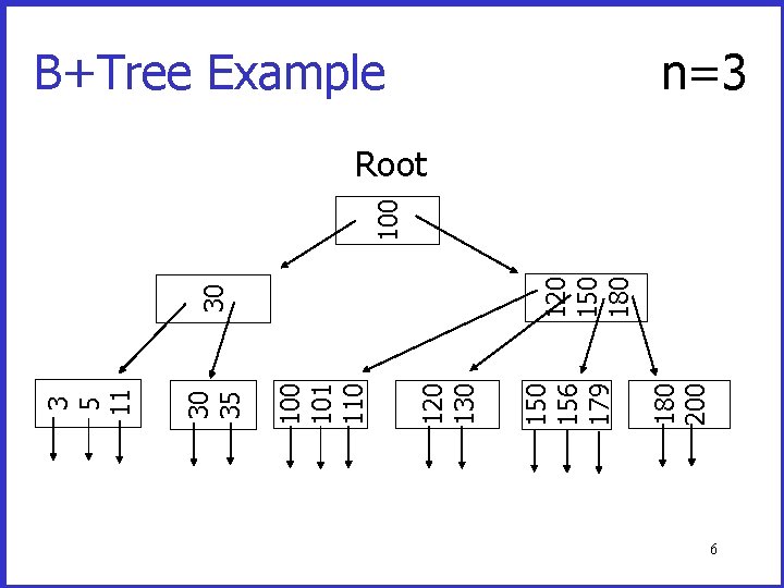
180 200 156 179 120 130 101 110 30 35 3 5 11 120 150 180 30 100 B+Tree Example n=3 Root 6

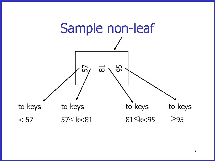
95 81 57 Sample non-leaf to keys < 57 57 k<81 81 k<95 to keys 95 7

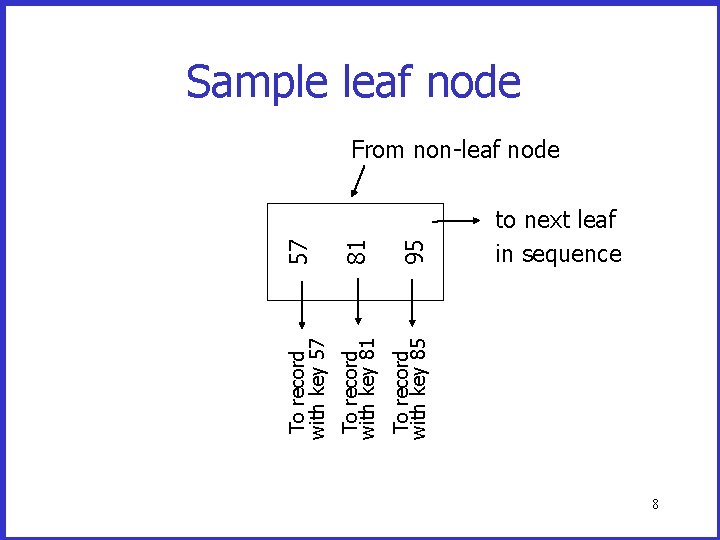
57 81 95 To record with key 57 To record with key 81 To record with key 85 Sample leaf node From non-leaf node to next leaf in sequence 8

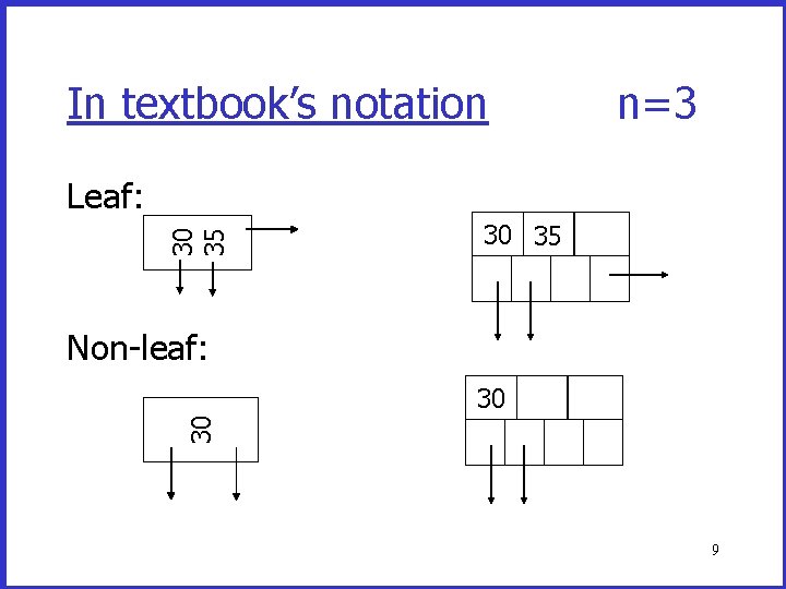
In textbook’s notation n=3 30 35 Leaf: 30 35 Non-leaf: 30 30 9

Maximal Sizes of Nodes Size of nodes: n+1 pointers (fixed) n keys • In leaf nodes, a pointer is associated with each key, and there is one additional pointer to the next leaf in sequential order • In non-leaf nodes, the leftmost pointer has no associated value 10

Don’t want nodes to be too empty • Use at least Non-leaf: (n+1)/2 pointers Leaf: (n+1)/2 pointers to data 11

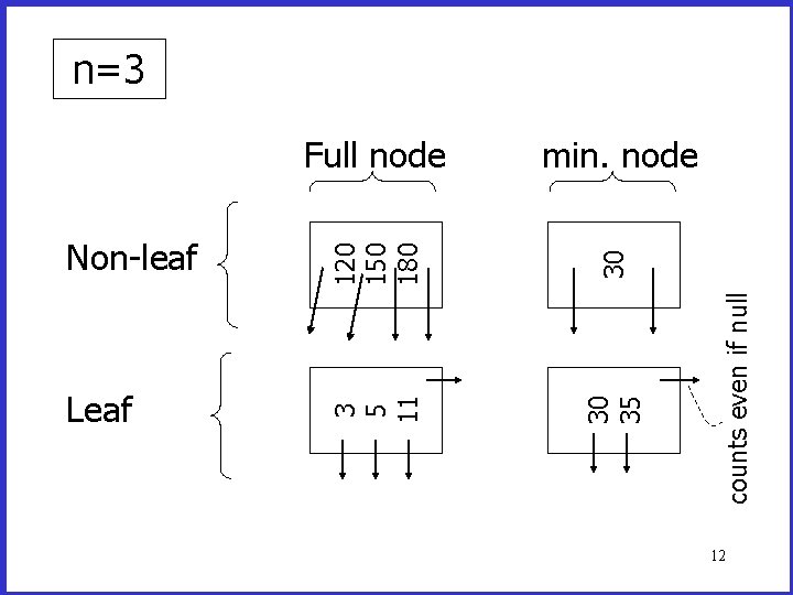
120 150 180 30 Leaf 30 35 Full node counts even if null Non-leaf 3 5 11 n=3 min. node 12

B+Tree Rules (tree of order n) (1) All leaves at same lowest level (balanced tree) (2) Pointers in leaves point to records except for “sequence pointer” Third rule on next slide 13

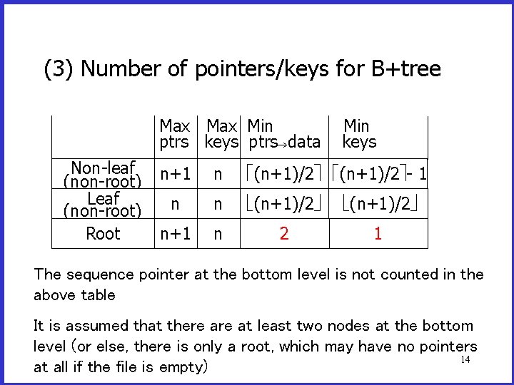
(3) Number of pointers/keys for B+tree Max Min ptrs keys ptrs data Non-leaf (non-root) Leaf (non-root) Root Min keys n+1 n (n+1)/2 - 1 n n (n+1)/2 n+1 n 2 1 The sequence pointer at the bottom level is not counted in the above table It is assumed that there at least two nodes at the bottom level (or else, there is only a root, which may have no pointers 14 at all if the file is empty)

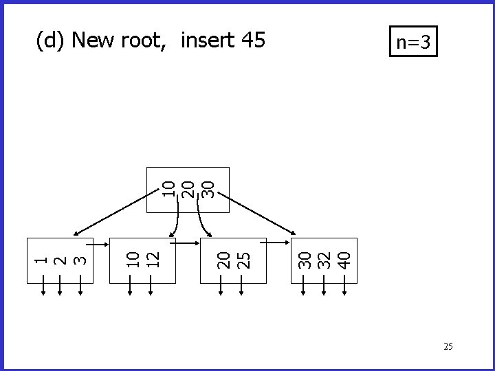
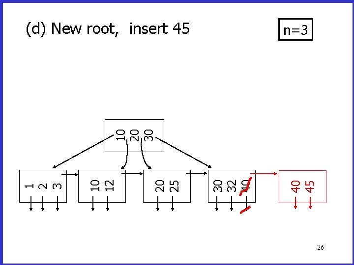
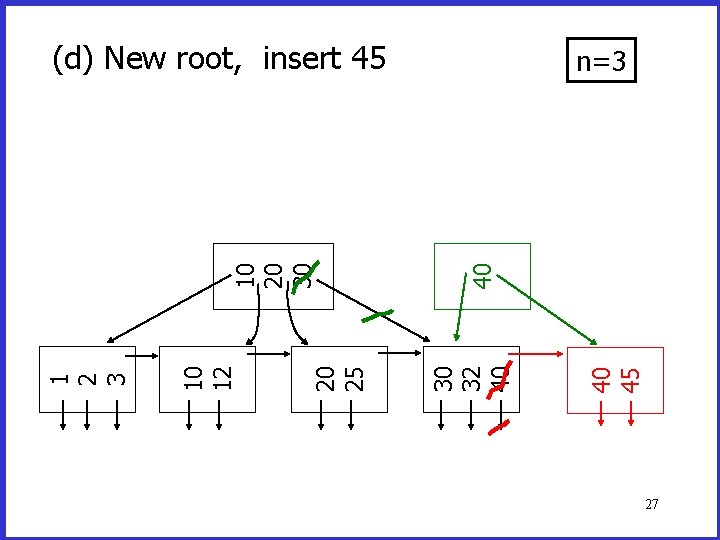
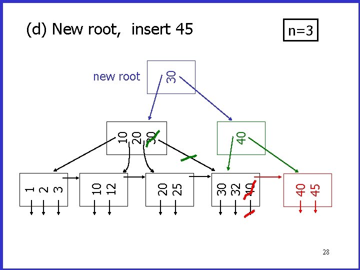
Insertion into a B+Tree (a) simple case – space available in leaf (b) leaf overflow (c) non-leaf overflow (d) new root 15

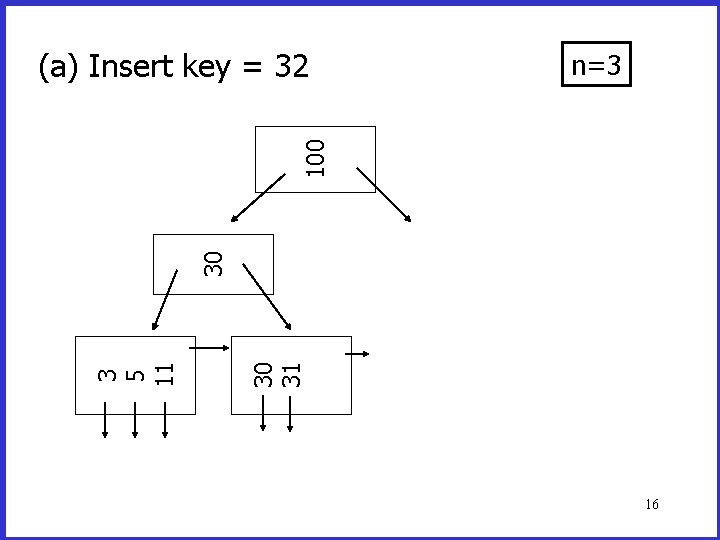
n=3 30 31 3 5 11 30 100 (a) Insert key = 32 16

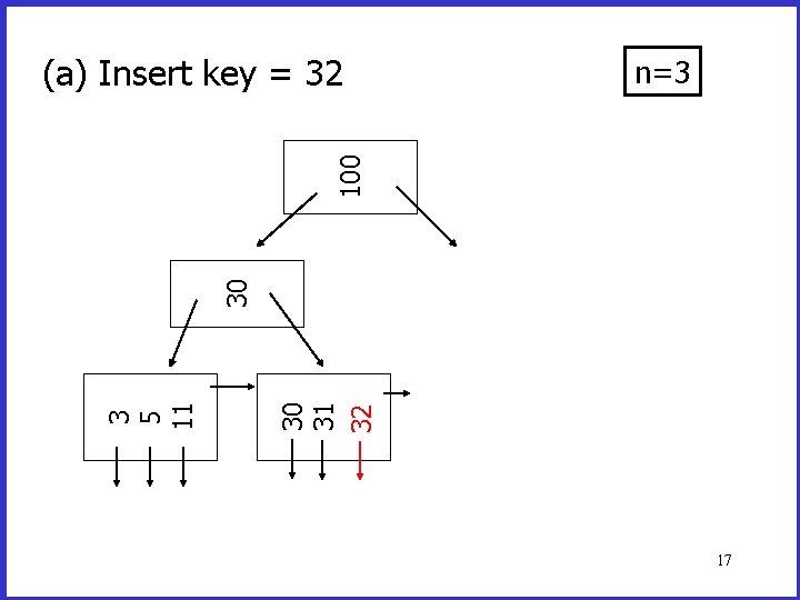
n=3 30 31 32 3 5 11 30 100 (a) Insert key = 32 17

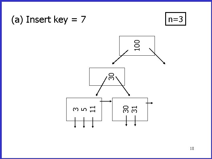
(a) Insert key = 7 30 31 3 5 11 30 100 n=3 18

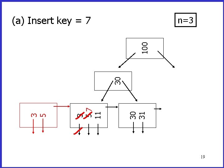
(a) Insert key = 7 30 31 3 57 11 3 5 30 100 n=3 19

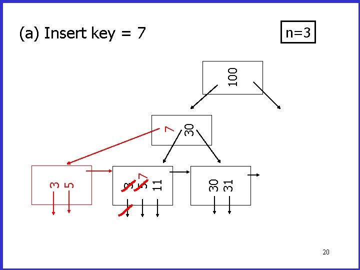
(a) Insert key = 7 30 30 31 3 57 11 3 5 7 100 n=3 20

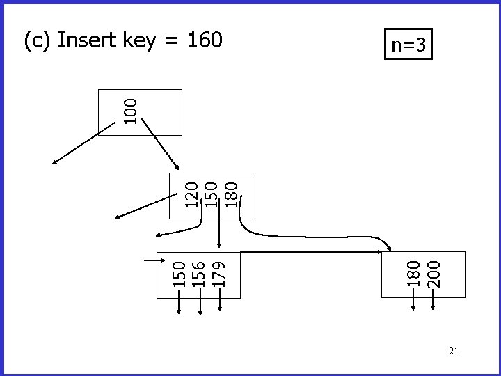
180 200 156 179 120 150 180 100 (c) Insert key = 160 n=3 21

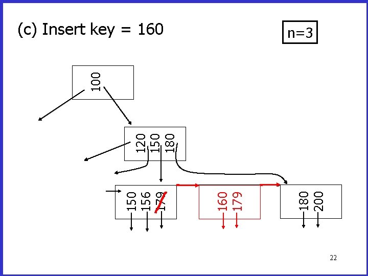
180 200 160 179 150 156 179 120 150 180 100 (c) Insert key = 160 n=3 22

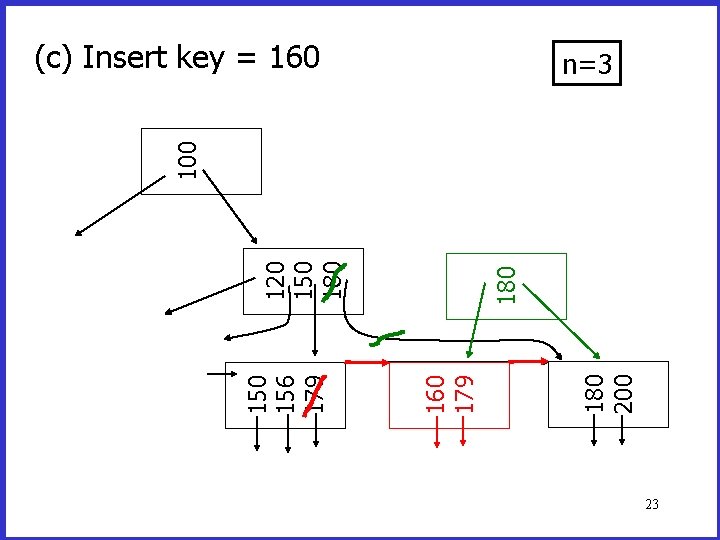
180 200 160 179 150 156 179 180 120 150 180 100 (c) Insert key = 160 n=3 23

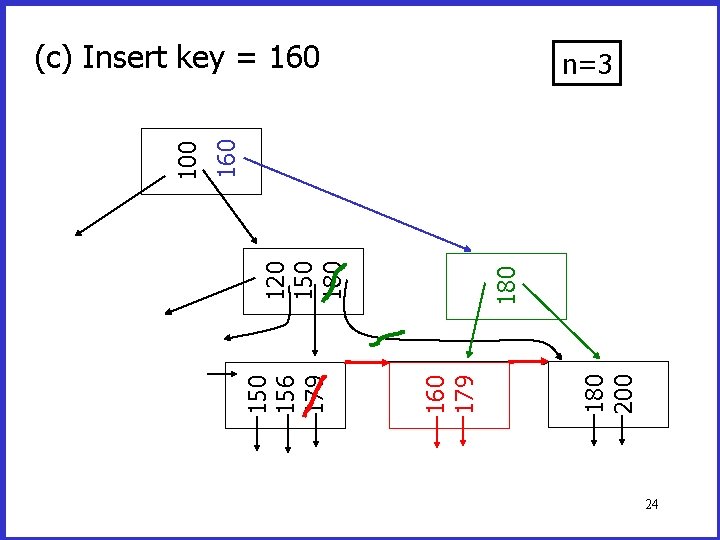
180 200 160 179 150 156 179 180 120 150 180 160 100 (c) Insert key = 160 n=3 24

(d) New root, insert 45 30 32 40 20 25 10 12 1 2 3 10 20 30 n=3 25

(d) New root, insert 45 40 45 30 32 40 20 25 10 12 1 2 3 10 20 30 n=3 26

40 45 30 32 40 20 25 10 12 1 2 3 40 10 20 30 (d) New root, insert 45 n=3 27

(d) New root, insert 45 40 30 32 40 20 25 10 12 1 2 3 10 20 30 30 new root n=3 28

Insertion Made Simple • View a node as a sorted list of pairs (k, p) – In a leaf, there is a pair (k, p) for each key and pointer associated with the same record • Ignore the sequence pointer to the next node – In a non-leaf node, (k, p) is created for each key and the pointer on its right side • The meaning of (k, p) is that p points to the subtree whose smallest key is k 29

What is the Pair for the Leftmost Pointer? • Create a virtual pair (k, p) for the leftmost pointer in each non-leaf node d – On the leftmost branch, k is - – In other non-leaf nodes, k is taken from the last proper (i. e. , non-virtual) pair that was used to reach d • The virtual pairs are created when traversing the path from the root to a leaf – For insertion, no need to create the virtual pairs 30

Insertion Process • We start by inserting a new pair (k, p) into a leaf • If a node d becomes overfull – Create a new node d’ on the right side of d, and – Move half of the pairs to the new node • If d’ is non-leaf, the key of its leftmost pair becomes virtual (i. e. , is deleted after the next step) • Create a pair (k’ , p’ ), where k’ is the smallest key in d’ and p’ is a pointer to d’ • Insert (k’ , p’ ) into the parent of d, on the right side of the pair that points to d – (k’ , p’ ) is never inserted in the leftmost position • If the parent of d becomes overfull, continue recursively (may have to create a new root eventually) 31

Deletion from a B+tree (a) Simple case - no example (b) Merge with neighbor (sibling) (c) Re-distribute keys (d) Cases (b) or (c) at non-leaf 32

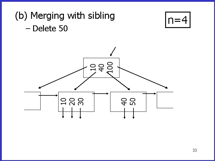
(b) Merging with sibling n=4 40 50 10 20 30 10 40 100 – Delete 50 33

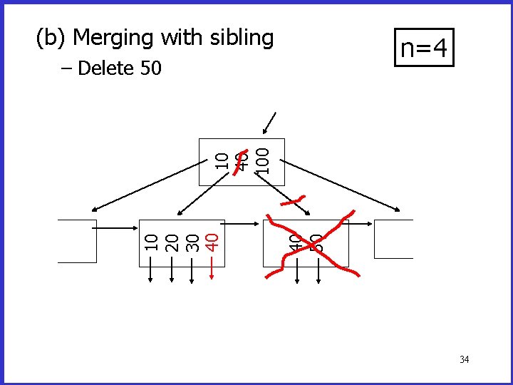
(b) Merging with sibling n=4 40 50 10 20 30 40 100 – Delete 50 34

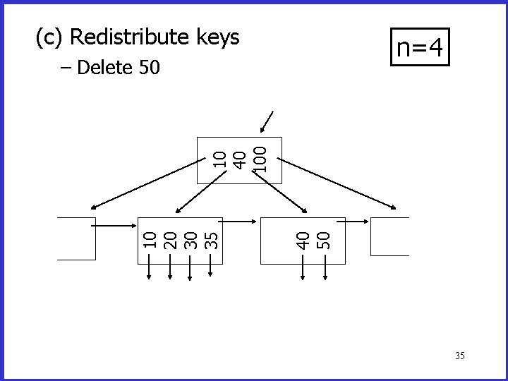
(c) Redistribute keys n=4 40 50 10 20 30 35 10 40 100 – Delete 50 35

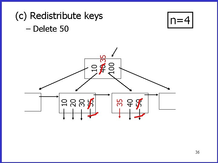
(c) Redistribute keys n=4 35 40 50 10 20 30 35 10 40 35 100 – Delete 50 36

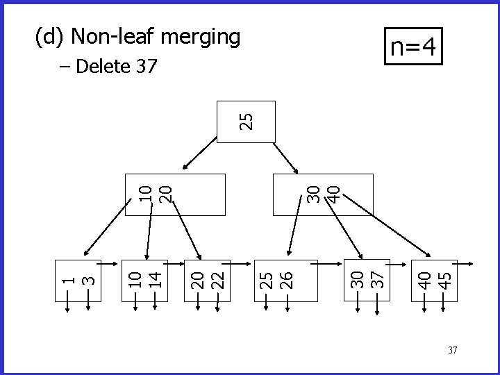
(d) Non-leaf merging n=4 40 45 30 37 30 40 25 26 20 22 10 14 1 3 10 20 25 – Delete 37 37

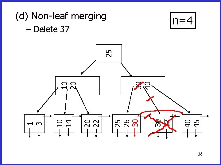
(d) Non-leaf merging n=4 40 45 30 37 30 40 25 26 30 20 22 10 14 1 3 10 20 25 – Delete 37 38

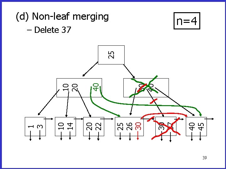
(d) Non-leaf merging n=4 40 45 30 37 30 40 25 26 30 40 20 22 10 14 1 3 10 20 25 – Delete 37 39

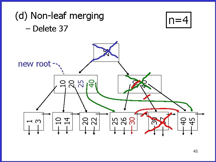
(d) Non-leaf merging n=4 25 – Delete 37 40 45 30 37 30 40 25 26 30 20 22 10 14 1 3 10 20 25 40 new root 40

B+Tree Deletions in Practice • Often, merging is not implemented – Too hard and not worth it! • Files usually grow in size over time 41

B+Trees as Search Keys • A B+Tree can implement either a primary or a secondary search key • If it is a secondary search key, then the leaves store the records of a one-level dense index, namely, – Pairs of a key and a pointer • If it is a primary search key, the leaves can store either a one-level index or the file itself – In the second option, the records are longer than those stored in non-leaf nodes – is it a problem? • Can the leaves store a sparse index? Answers on next slide 42

Suppose that a B+tree is a primary search key • If the file is stored separately and is sorted on the primary key, then the bottom level of the B+tree is a one-level sparse index • If the file is stored separately, but is not sorted (i. e. , the file is a heap), then the bottom level must be a one-level dense index • If the file is stored in the leaves of the B+tree, then the records in the leaves are longer than those in the non-leaf nodes – The parameter n (which determines the max and min number of records in the nodes) is different in the leaves (i. e. , it is smaller than in the non-leaf nodes) 43

B+Trees vs. Dense & Sparse Indexes • D & S indexes could be more efficient if – When creating or reorganizing, we leave enough space for future insertions • But we should not leave too much space or else we’ll hurt performance – We reorganize before performance deteriorates too much • But it is hard to know how much free space to leave and when to reorganize – Hence, B+trees are more efficient in practice 44

Buffering Requirements • Since B+trees have no overflow blocks, they need to look at only one block from each level • D & S indexes require larger and variable-size buffer space • Also, only after reading a block, can we determine whether an overflow block also has to be read (and that overflow block is unlikely to be contiguous with the first block) – Render read-ahead buffering ineffective • BTW, is LRU good for B+trees? 45

B Tree: A Variation on a B+Tree • In a B Tree, some of the records (of the index or the file) are stored in non-leaf nodes – Why is it a good idea? • Disadvantage of B trees – Two sizes of records in non-leaf nodes • For fixed-sized blocks, fanout of non-leaf nodes is smaller; hence, tree is deeper and lookup takes longer – Deletion is more complicated – Hard to chain the records (of the index or the file) 46