Query Processing Optimization John Ortiz Lecture 19 Query

Query Processing & Optimization John Ortiz Lecture 19 Query Processing & Optimization

Terms ® DBMS has algorithms to implement relational algebra expressions ® SQL is a different kind of high level language; specify what is wanted, not how it is obtained ® Optimization – not necessarily “optimal”, but reasonably efficient ® Techniques: æHeuristic rules æCost estimation Lecture 19 Query Processing & Optimization 2

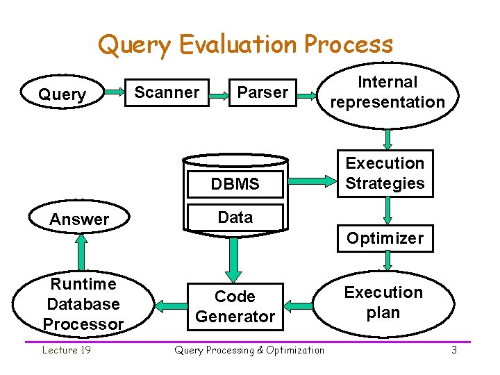
Query Evaluation Process Query Scanner Parser DBMS Answer Internal representation Execution Strategies Data Optimizer Runtime Database Processor Lecture 19 Code Generator Query Processing & Optimization Execution plan 3

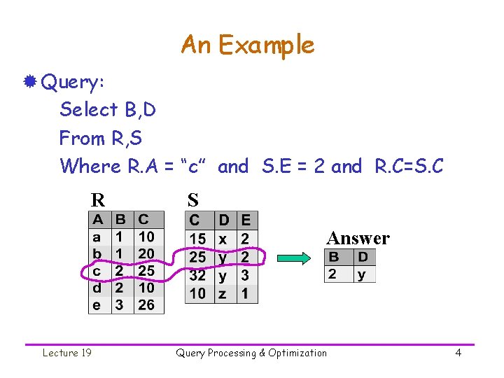
An Example ® Query: Select B, D From R, S Where R. A = “c” and S. E = 2 and R. C=S. C R S Answer Lecture 19 Query Processing & Optimization 4

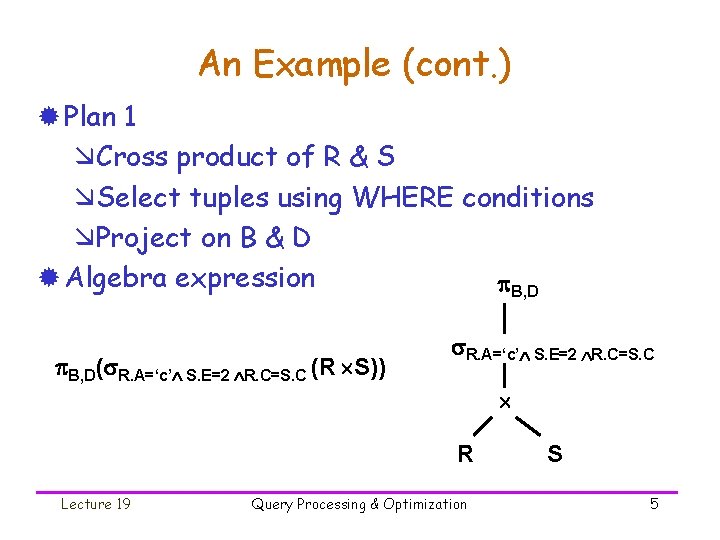
An Example (cont. ) ® Plan 1 æCross product of R & S æSelect tuples using WHERE conditions æProject on B & D ® Algebra expression B, D( R. A=‘c’ S. E=2 R. C=S. C (R S)) R. A=‘c’ S. E=2 R. C=S. C R Lecture 19 Query Processing & Optimization S 5

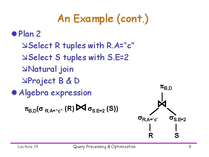
An Example (cont. ) ® Plan 2 æSelect R tuples with R. A=“c” æSelect S tuples with S. E=2 æNatural join æProject B & D ® Algebra expression B, D( R. A=“c” (R) S. E=2 (S)) B, D R. A=‘c’ R Lecture 19 Query Processing & Optimization S. E=2 S 6

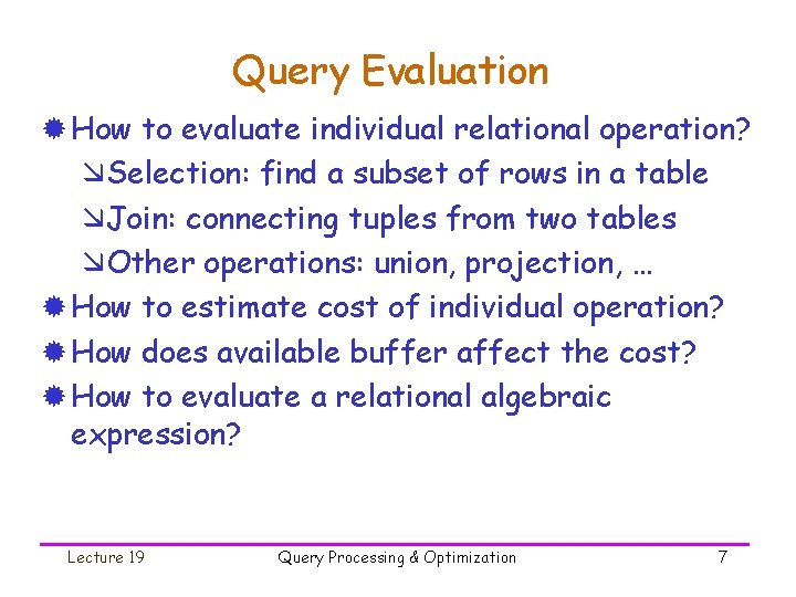
Query Evaluation ® How to evaluate individual relational operation? æSelection: find a subset of rows in a table æJoin: connecting tuples from two tables æOther operations: union, projection, … ® How to estimate cost of individual operation? ® How does available buffer affect the cost? ® How to evaluate a relational algebraic expression? Lecture 19 Query Processing & Optimization 7

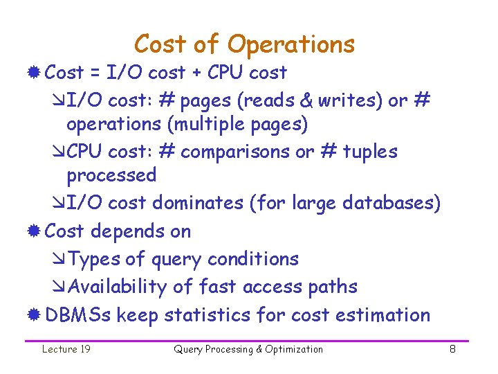
Cost of Operations ® Cost = I/O cost + CPU cost æI/O cost: # pages (reads & writes) or # operations (multiple pages) æCPU cost: # comparisons or # tuples processed æI/O cost dominates (for large databases) ® Cost depends on æTypes of query conditions æAvailability of fast access paths ® DBMSs keep statistics for cost estimation Lecture 19 Query Processing & Optimization 8

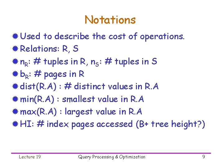
Notations ® Used to describe the cost of operations. ® Relations: R, S ® n. R: # tuples in R, n. S: # tuples in S ® b. R: # pages in R ® dist(R. A) : # distinct values in R. A ® min(R. A) : smallest value in R. A ® max(R. A) : largest value in R. A ® HI: # index pages accessed (B+ tree height? ) Lecture 19 Query Processing & Optimization 9

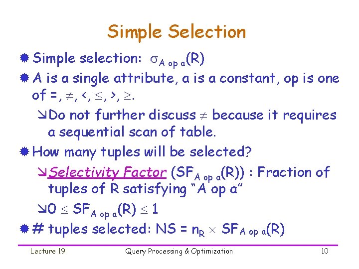
Simple Selection ® Simple selection: A op a(R) ® A is a single attribute, a is a constant, op is one of =, , <, , >, . æDo not further discuss because it requires a sequential scan of table. ® How many tuples will be selected? æSelectivity Factor (SFA op a(R)) : Fraction of tuples of R satisfying “A op a” æ 0 SFA op a(R) 1 ® # tuples selected: NS = n. R SFA op a(R) Lecture 19 Query Processing & Optimization 10

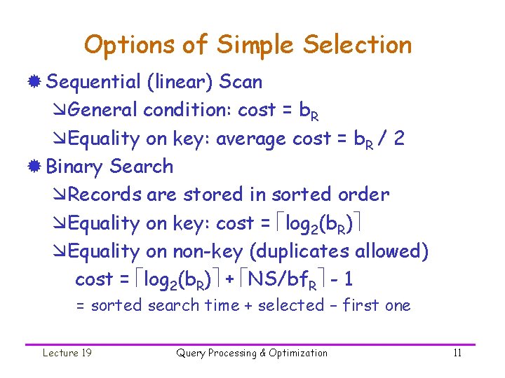
Options of Simple Selection ® Sequential (linear) Scan æGeneral condition: cost = b. R æEquality on key: average cost = b. R / 2 ® Binary Search æRecords are stored in sorted order æEquality on key: cost = log 2(b. R) æEquality on non-key (duplicates allowed) cost = log 2(b. R) + NS/bf. R - 1 = sorted search time + selected – first one Lecture 19 Query Processing & Optimization 11

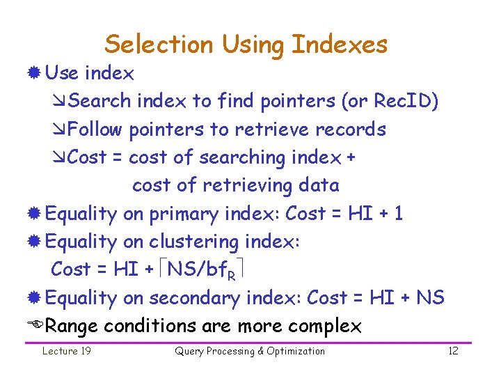
Selection Using Indexes ® Use index æSearch index to find pointers (or Rec. ID) æFollow pointers to retrieve records æCost = cost of searching index + cost of retrieving data ® Equality on primary index: Cost = HI + 1 ® Equality on clustering index: Cost = HI + NS/bf. R ® Equality on secondary index: Cost = HI + NS ERange conditions are more complex Lecture 19 Query Processing & Optimization 12

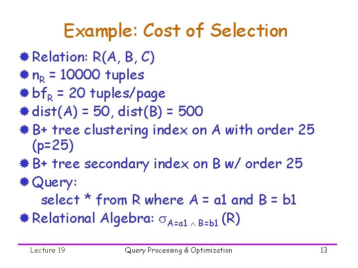
Example: Cost of Selection ® Relation: R(A, B, C) ® n. R = 10000 tuples ® bf. R = 20 tuples/page ® dist(A) = 50, dist(B) = 500 ® B+ tree clustering index on A with order 25 (p=25) ® B+ tree secondary index on B w/ order 25 ® Query: select * from R where A = a 1 and B = b 1 ® Relational Algebra: A=a 1 B=b 1 (R) Lecture 19 Query Processing & Optimization 13

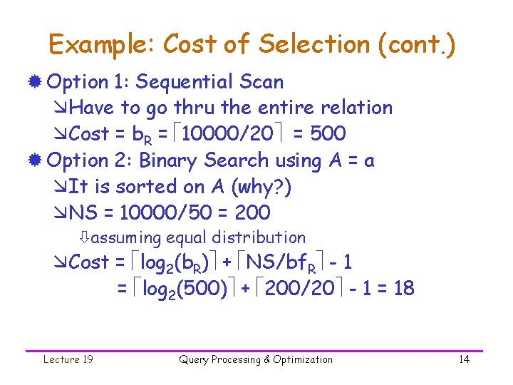
Example: Cost of Selection (cont. ) ® Option 1: Sequential Scan æHave to go thru the entire relation æCost = b. R = 10000/20 = 500 ® Option 2: Binary Search using A = a æIt is sorted on A (why? ) æNS = 10000/50 = 200 òassuming equal distribution æCost = log 2(b. R) + NS/bf. R - 1 = log 2(500) + 200/20 - 1 = 18 Lecture 19 Query Processing & Optimization 14

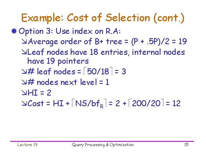
Example: Cost of Selection (cont. ) ® Option 3: Use index on R. A: æAverage order of B+ tree = (P +. 5 P)/2 = 19 æLeaf nodes have 18 entries, internal nodes have 19 pointers æ# leaf nodes = 50/18 = 3 æ# nodes next level = 1 æHI = 2 æCost = HI + NS/bf. R = 2 + 200/20 = 12 Lecture 19 Query Processing & Optimization 15

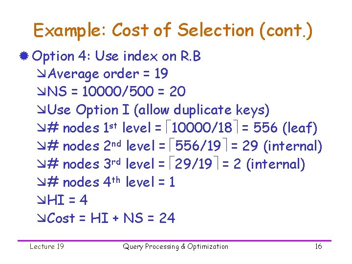
Example: Cost of Selection (cont. ) ® Option 4: Use index on R. B æAverage order = 19 æNS = 10000/500 = 20 æUse Option I (allow duplicate keys) æ# nodes 1 st level = 10000/18 = 556 (leaf) æ# nodes 2 nd level = 556/19 = 29 (internal) æ# nodes 3 rd level = 29/19 = 2 (internal) æ# nodes 4 th level = 1 æHI = 4 æCost = HI + NS = 24 Lecture 19 Query Processing & Optimization 16

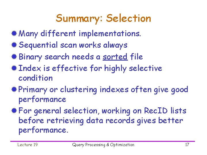
Summary: Selection ® Many different implementations. ® Sequential scan works always ® Binary search needs a sorted file ® Index is effective for highly selective condition ® Primary or clustering indexes often give good performance ® For general selection, working on Rec. ID lists before retrieving data records gives better performance. Lecture 19 Query Processing & Optimization 17

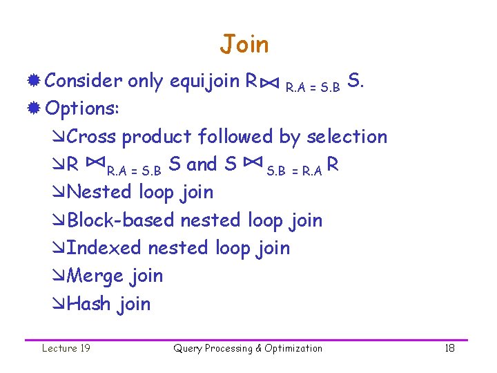
Join ® Consider only equijoin R R. A = S. B S. ® Options: æCross product followed by selection æR R. A = S. B S and S S. B = R. A R æNested loop join æBlock-based nested loop join æIndexed nested loop join æMerge join æHash join Lecture 19 Query Processing & Optimization 18

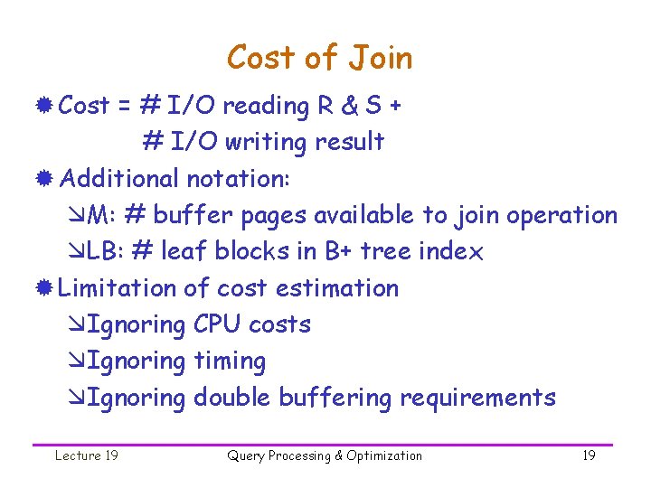
Cost of Join ® Cost = # I/O reading R & S + # I/O writing result ® Additional notation: æM: # buffer pages available to join operation æLB: # leaf blocks in B+ tree index ® Limitation of cost estimation æIgnoring CPU costs æIgnoring timing æIgnoring double buffering requirements Lecture 19 Query Processing & Optimization 19

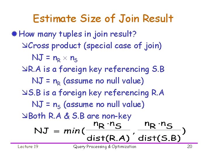
Estimate Size of Join Result ® How many tuples in join result? æCross product (special case of join) NJ = n. R n. S æR. A is a foreign key referencing S. B NJ = n. R (assume no null value) æS. B is a foreign key referencing R. A NJ = n. S (assume no null value) æBoth R. A & S. B are non-key Lecture 19 Query Processing & Optimization 20

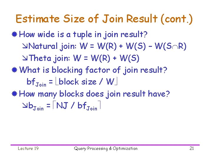
Estimate Size of Join Result (cont. ) ® How wide is a tuple in join result? æNatural join: W = W(R) + W(S) – W(S R) æTheta join: W = W(R) + W(S) ® What is blocking factor of join result? bf. Join = block size / W ® How many blocks does join result have? æb. Join = NJ / bf. Join Lecture 19 Query Processing & Optimization 21

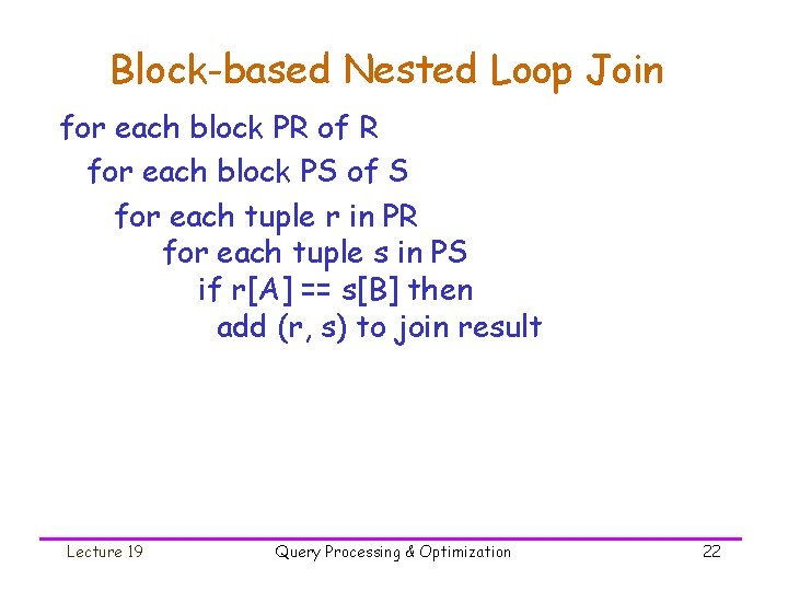
Block-based Nested Loop Join for each block PR of R for each block PS of S for each tuple r in PR for each tuple s in PS if r[A] == s[B] then add (r, s) to join result Lecture 19 Query Processing & Optimization 22

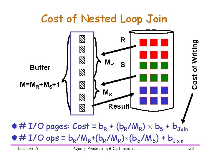
R Buffer M=MR+MS+1 MR S MS Cost of Writing Cost of Nested Loop Join Result ® # I/O pages: Cost = b. R + (b. R/MR) b. S + b. Join ® # I/O ops = b. R/MR+(b. R/MR) (b. S/MS) + b. Join Lecture 19 Query Processing & Optimization 23

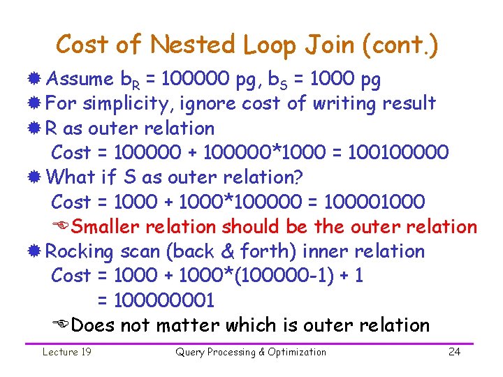
Cost of Nested Loop Join (cont. ) ® Assume b. R = 100000 pg, b. S = 1000 pg ® For simplicity, ignore cost of writing result ® R as outer relation Cost = 100000 + 100000*1000 = 100100000 ® What if S as outer relation? Cost = 1000 + 1000*100000 = 100001000 ESmaller relation should be the outer relation ® Rocking scan (back & forth) inner relation Cost = 1000 + 1000*(100000 -1) + 1 = 100000001 EDoes not matter which is outer relation Lecture 19 Query Processing & Optimization 24

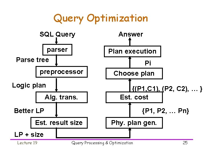
Query Optimization SQL Query parser Parse tree Answer Plan execution Pi preprocessor Logic plan Alg. trans. Choose plan {(P 1, C 1), (P 2, C 2), … } Est. cost Better LP {P 1, P 2, … Pn} Est. result size Phy. plan gen. LP + size Lecture 19 Query Processing & Optimization 25

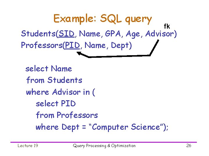
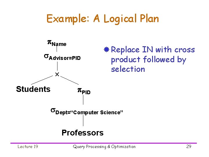
Example: SQL query fk Students(SID, Name, GPA, Age, Advisor) Professors(PID, Name, Dept) select Name from Students where Advisor in ( select PID from Professors where Dept = “Computer Science”); Lecture 19 Query Processing & Optimization 26

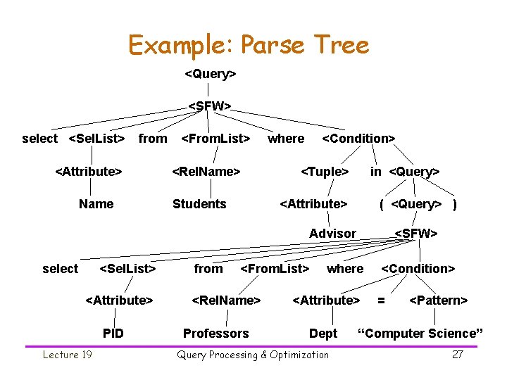
Example: Parse Tree <Query> <SFW> select <Sel. List> from <Attribute> Name <From. List> <Rel. Name> Students where <Condition> <Tuple> in <Query> <Attribute> ( <Query> ) Advisor select <Sel. List> <Attribute> PID Lecture 19 from <From. List> <Rel. Name> Professors <SFW> where <Attribute> Dept Query Processing & Optimization <Condition> = <Pattern> “Computer Science” 27

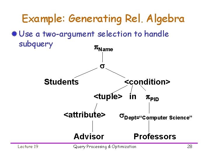
Example: Generating Rel. Algebra ® Use a two-argument selection to handle subquery Name Students <condition> <tuple> in <attribute> Advisor Lecture 19 PID Dept=“Computer Science” Professors Query Processing & Optimization 28

Example: A Logical Plan Name Advisor=PID Students ® Replace IN with cross product followed by selection PID Dept=“Computer Science” Professors Lecture 19 Query Processing & Optimization 29

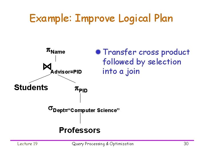
Example: Improve Logical Plan Name Advisor=PID Students ® Transfer cross product followed by selection into a join PID Dept=“Computer Science” Professors Lecture 19 Query Processing & Optimization 30

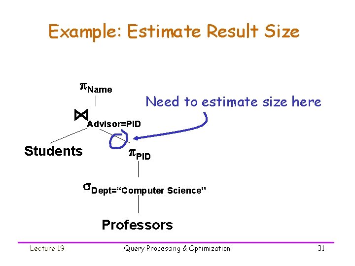
Example: Estimate Result Size Name Need to estimate size here Advisor=PID Students PID Dept=“Computer Science” Professors Lecture 19 Query Processing & Optimization 31

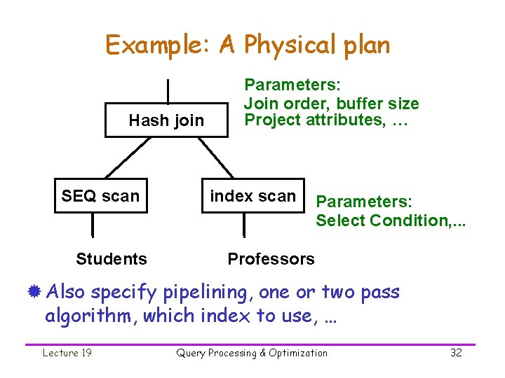
Example: A Physical plan Hash join SEQ scan Students Parameters: Join order, buffer size Project attributes, … index scan Parameters: Select Condition, . . . Professors ® Also specify pipelining, one or two pass algorithm, which index to use, … Lecture 19 Query Processing & Optimization 32

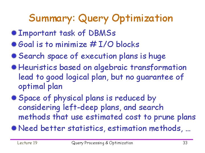
Summary: Query Optimization ® Important task of DBMSs ® Goal is to minimize # I/O blocks ® Search space of execution plans is huge ® Heuristics based on algebraic transformation lead to good logical plan, but no guarantee of optimal plan ® Space of physical plans is reduced by considering left-deep plans, and search methods that use estimated cost to prune plans ® Need better statistics, estimation methods, … Lecture 19 Query Processing & Optimization 33