Query Processing COMP 3017 Advanced Databases Nicholas Gibbins

Query Processing COMP 3017 Advanced Databases Nicholas Gibbins - nmg@ecs. soton. ac. uk 2012 -2013
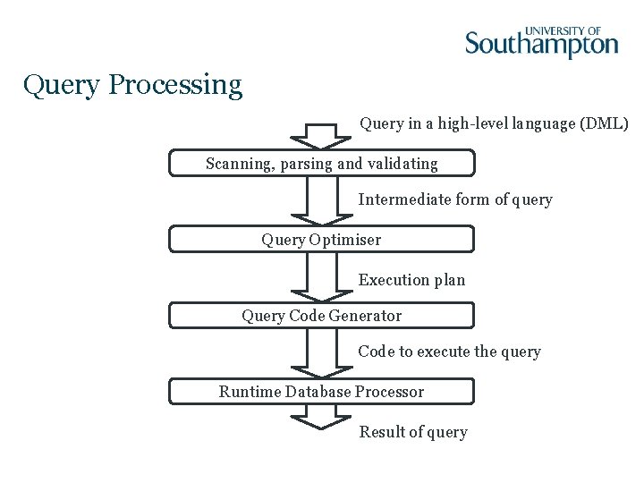
Query Processing Query in a high-level language (DML) Scanning, parsing and validating Intermediate form of query Query Optimiser Execution plan Query Code Generator Code to execute the query Runtime Database Processor Result of query
Query Plans Logical Query Plan – algebraic representation of query – operators taken from relational algebra – abstract! Physical Query Plan – algorithms selected for each operator in plan – execution order specified for operators
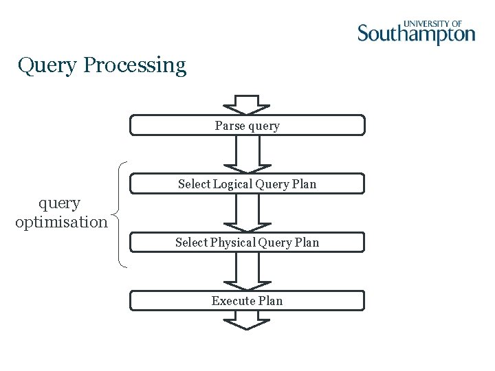
Query Processing Parse query Select Logical Query Plan query optimisation Select Physical Query Plan Execute Plan

Query Processing Parse query Select Logical Query Plan Generate Logical Query Plan Rewrite Logical Query Plan Select Physical Query Plan Execute Plan
This Week Physical query plans Logical query plans - Physical query plan operators - Improving logical query plans - One-pass algorithms - Cost estimation - Nested-loop joins - Cost-based plan selection - Two-pass algorithms - Join ordering - Index-based algorithms

Physical-Plan Operators
Physical-Plan Operators Algorithm that implements one of the basic relational operations that are used in query plans For example, relational algebra has join operator How that join is carried out depends on: – structure of relations – size of relations – presence of indexes and hashes –. . .
Computation Model Need to choose good physical-plan operators – Estimate the “cost” of each operator – Key measure of cost is the number of disk accesses (far more costly than main memory accesses) Assumption: arguments of operator are on disk, result is in main memory
Cost Parameters M: Main memory available for buffers S(R): Size of a tuple of relation R B(R): Blocks used to store relation R T(R): Number of tuples in relation R (cardinality of R) V(R, a): Number of distinct values for attribute a in relation R
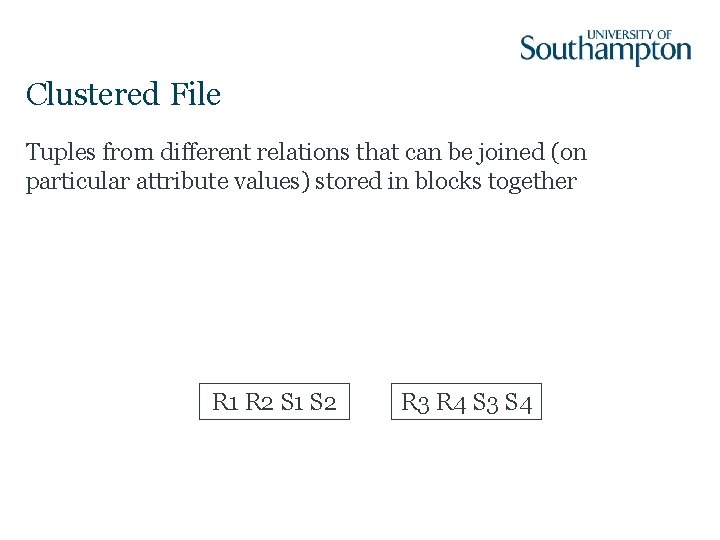
Clustered File Tuples from different relations that can be joined (on particular attribute values) stored in blocks together R 1 R 2 S 1 S 2 R 3 R 4 S 3 S 4
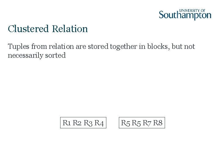
Clustered Relation Tuples from relation are stored together in blocks, but not necessarily sorted R 1 R 2 R 3 R 4 R 5 R 7 R 8
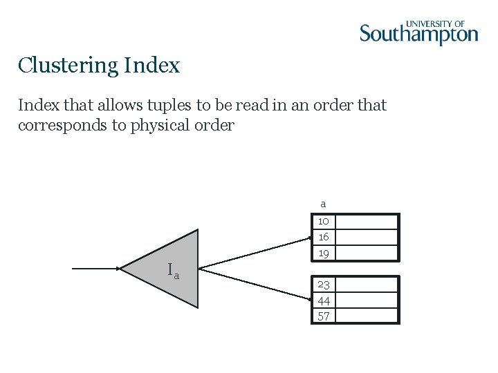
Clustering Index that allows tuples to be read in an order that corresponds to physical order a 10 16 19 Ia 23 44 57

Scanning
Scan • Read all of the tuples of a relation R • Read only those tuples of a relation R that satisfy some predicate Two variants: – Table scan – Index scan
Table Scan Tuples arranged in blocks – All blocks known to the system – Possible to get blocks one at a time I/O Cost – B(R) disk accesses, if R is clustered – T(R) disk accesses, if R is not clustered
Index Scan An index exists on some attribute of R – Use index to find all blocks holding R – Retrieve blocks for R I/O Cost – B(R) + B(IR) disk accesses if clustered – B(R) >> B(IR), so treat as only B(R) – T(R) disk accesses if not clustered

One-Pass Algorithms
One-Pass Algorithms • Read data from disk only once • Typically require that at least one argument fits in main memory • Three broad categories: – Unary, tuple at a time (i. e. select, project) – Unary, full-relation (i. e. duplicate elimination, grouping) – Binary, full-relation
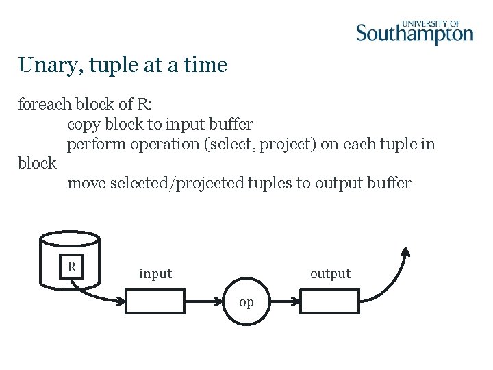
Unary, tuple at a time foreach block of R: copy block to input buffer perform operation (select, project) on each tuple in block move selected/projected tuples to output buffer R input output op
Unary, tuple at a time: Cost In general, B(R) or T(R) disk accesses depending on clustering If operator is a select that compares an attribute to a constant and index exists for attributes used in select, <<B(R) disk accesses Requires M>=1
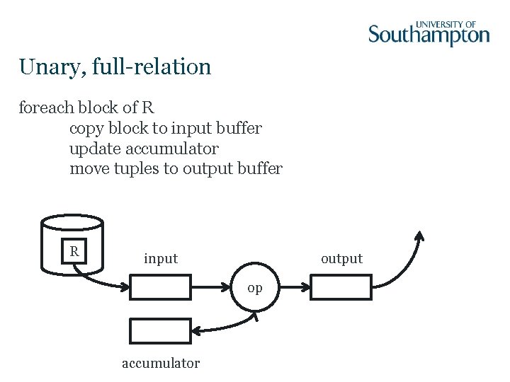
Unary, full-relation foreach block of R copy block to input buffer update accumulator move tuples to output buffer R input output op accumulator
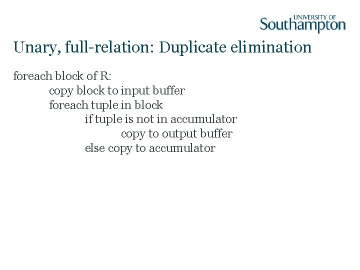
Unary, full-relation: Duplicate elimination foreach block of R: copy block to input buffer foreach tuple in block if tuple is not in accumulator copy to output buffer else copy to accumulator
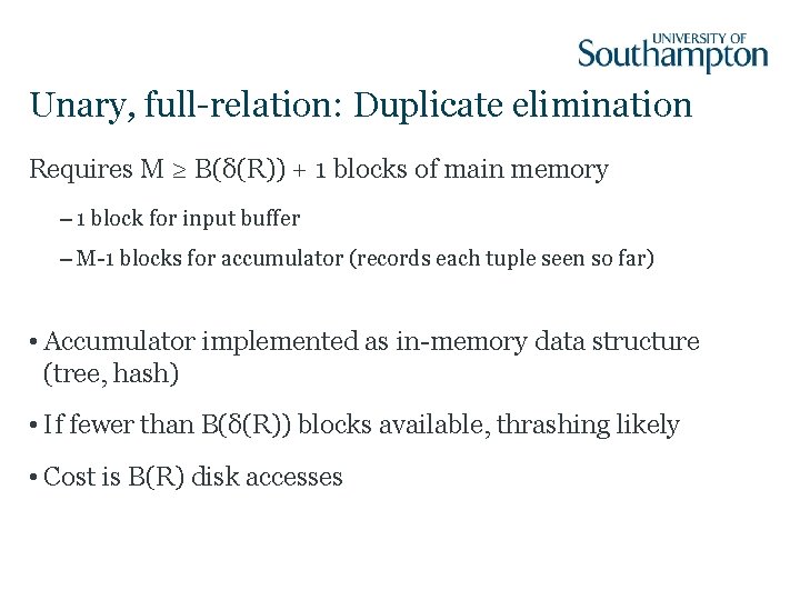
Unary, full-relation: Duplicate elimination Requires M ≥ B(δ(R)) + 1 blocks of main memory – 1 block for input buffer – M-1 blocks for accumulator (records each tuple seen so far) • Accumulator implemented as in-memory data structure (tree, hash) • If fewer than B(δ(R)) blocks available, thrashing likely • Cost is B(R) disk accesses
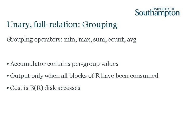
Unary, full-relation: Grouping operators: min, max, sum, count, avg • Accumulator contains per-group values • Output only when all blocks of R have been consumed • Cost is B(R) disk accesses
Binary, full-relation Union, intersection, difference, product, join – We’ll consider join in detail In general, cost is B(R) + B(S) – R, S are operand relations Requirement for one pass operation: min(B(R), B(S)) ≤ M-1
Binary, full-relation: Join • Two relations, R(X, Y) and S(Y, Z), B(S)<B(R) • Uses main memory search structure keyed on Y foreach block of S: read block add tuples to search structure foreach block of R copy block to input buffer foreach tuple in block find matching tuples in search structure construct new tuples and copy to output

Nested-Loop Joins
Nested-loop join Also known as iteration join Assuming that we’re joining relations R, S on attribute C: foreach tuple r in R foreach tuple s in S if r. C = s. C then output r, s pair
Factors that affect cost • Tuples of relation stored physically together? (clustered) • Relations sorted by join attribute? • Indexes exist?
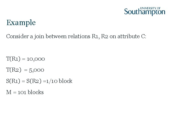
Example Consider a join between relations R 1, R 2 on attribute C: T(R 1) = 10, 000 T(R 2) = 5, 000 S(R 1) = S(R 2) =1/10 block M = 101 blocks
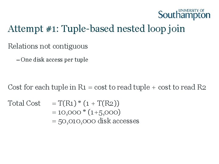
Attempt #1: Tuple-based nested loop join Relations not contiguous – One disk access per tuple Cost for each tuple in R 1 = cost to read tuple + cost to read R 2 Total Cost = T(R 1) * (1 + T(R 2)) = 10, 000 * (1+5, 000) = 50, 010, 000 disk accesses
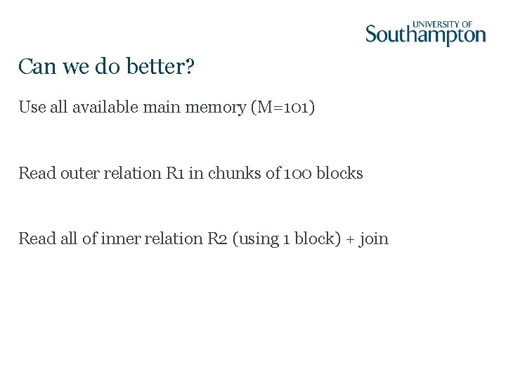
Can we do better? Use all available main memory (M=101) Read outer relation R 1 in chunks of 100 blocks Read all of inner relation R 2 (using 1 block) + join
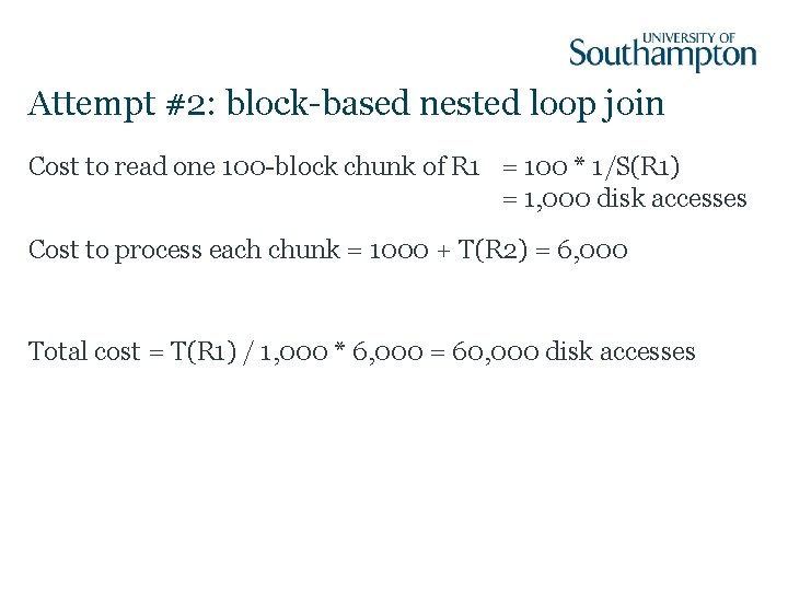
Attempt #2: block-based nested loop join Cost to read one 100 -block chunk of R 1 = 100 * 1/S(R 1) = 1, 000 disk accesses Cost to process each chunk = 1000 + T(R 2) = 6, 000 Total cost = T(R 1) / 1, 000 * 6, 000 = 60, 000 disk accesses
Can we do better? What happens if we reverse the join order? – R 1 becomes the inner relation – R 2 becomes the outer relation
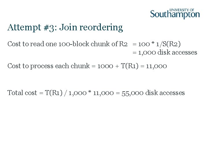
Attempt #3: Join reordering Cost to read one 100 -block chunk of R 2 = 100 * 1/S(R 2) = 1, 000 disk accesses Cost to process each chunk = 1000 + T(R 1) = 11, 000 Total cost = T(R 1) / 1, 000 * 11, 000 = 55, 000 disk accesses
Can we do better? What happens if the tuples in each relation are contiguous (i. e. clustered)
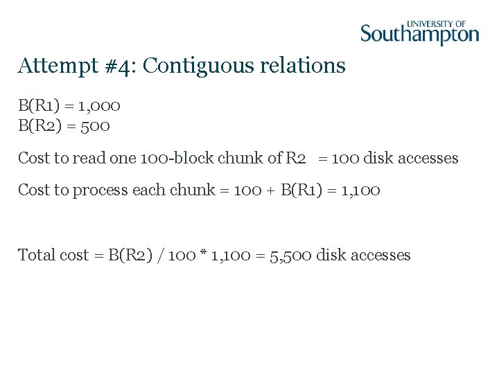
Attempt #4: Contiguous relations B(R 1) = 1, 000 B(R 2) = 500 Cost to read one 100 -block chunk of R 2 = 100 disk accesses Cost to process each chunk = 100 + B(R 1) = 1, 100 Total cost = B(R 2) / 100 * 1, 100 = 5, 500 disk accesses
Can we do better? What happens if both relations are contiguous and sorted by C, the join attribute?
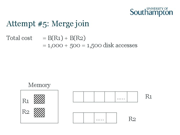
Attempt #5: Merge join Total cost = B(R 1) + B(R 2) = 1, 000 + 500 = 1, 500 disk accesses Memory R 1 R 2 R 1 …. . R 2

Two-Pass Algorithms
Can we do better? What if R 1 and R 2 aren’t sorted by C? . . . need to sort R 1 and R 2 first
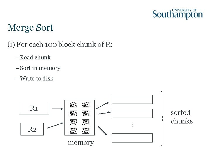
Merge Sort (i) For each 100 block chunk of R: – Read chunk – Sort in memory – Write to disk . . . R 1 R 2 memory sorted chunks
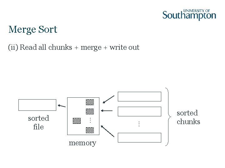
Merge Sort memory . . . sorted file . . . (ii) Read all chunks + merge + write out sorted chunks
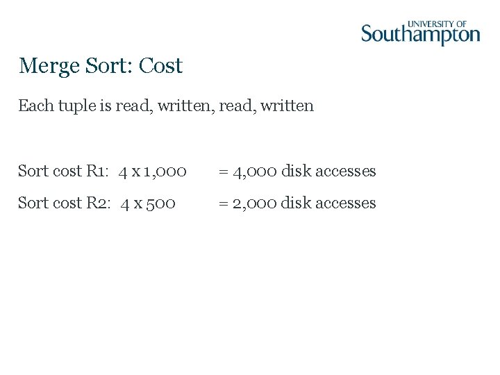
Merge Sort: Cost Each tuple is read, written, read, written Sort cost R 1: 4 x 1, 000 = 4, 000 disk accesses Sort cost R 2: 4 x 500 = 2, 000 disk accesses
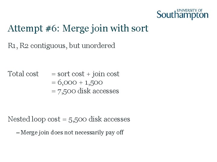
Attempt #6: Merge join with sort R 1, R 2 contiguous, but unordered Total cost = sort cost + join cost = 6, 000 + 1, 500 = 7, 500 disk accesses Nested loop cost = 5, 500 disk accesses – Merge join does not necessarily pay off
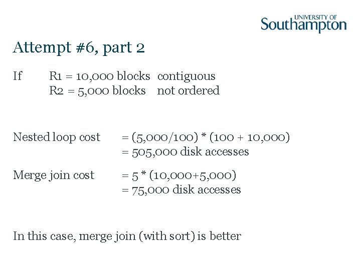
Attempt #6, part 2 If R 1 = 10, 000 blocks contiguous R 2 = 5, 000 blocks not ordered Nested loop cost = (5, 000/100) * (100 + 10, 000) = 505, 000 disk accesses Merge join cost = 5 * (10, 000+5, 000) = 75, 000 disk accesses In this case, merge join (with sort) is better
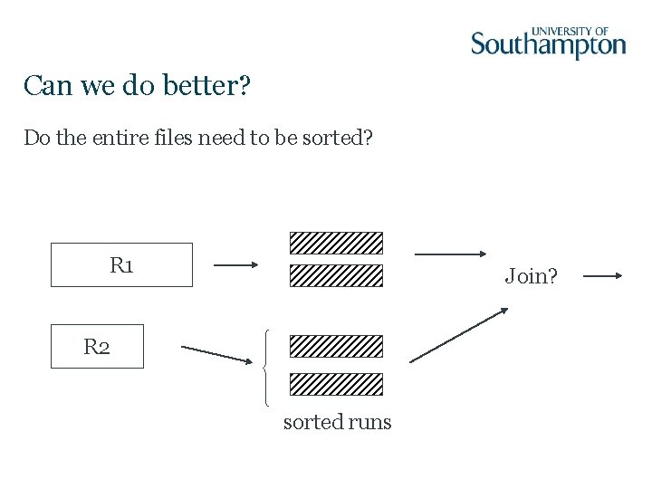
Can we do better? Do the entire files need to be sorted? R 1 Join? R 2 sorted runs
Attempt #7: Improved merge join 1. Read R 1 + write R 1 into runs 2. Read R 2 + write R 2 into runs 3. Merge join Total cost = 2, 000 + 1, 500 = 4, 500 disk accesses
Two-pass Algorithms using Hashing Partition relation into M-1 buckets In general: – Read relation a tuple at a time – Hash tuple to bucket – When bucket is full, move to disk and reinitialise bucket
Hash-Join The tuples in R and S are both hashed using the same hashing function on the join attributes 1. Read R 1 and write into buckets 2. Read R 2 and write into buckets 3. Join R 1, R 2 Total cost = 3 * (B(R 1) + B(R 2)) = 3 * (1, 000 + 500) = 4, 500 disk accesses

Index-based Algorithms
Can we do better? What if we have an index on the join attribute? • Assume R 1. C index exists; 2 levels • Assume R 2 contiguous, unordered • Assume R 1. C index fits in memory
Attempt #8: Index join Cost: Reads: 500 disk accesses foreach R 2 tuple: – probe index – free – if match, read R 1 tuple: 1 disk access
How many matching tuples? (a) If R 1. C is key, R 2. C is foreign key expected number of matching tuples = 1
How many matching tuples? (b) If V(R 1, C) = 5000, T(R 1) = 10, 000 and uniform assumption, expected matching tuples = 10, 000/5, 000 = 2
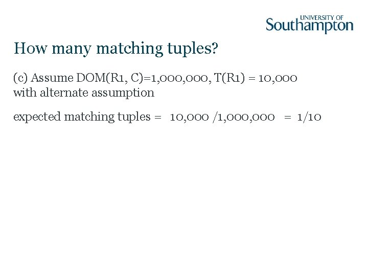
How many matching tuples? (c) Assume DOM(R 1, C)=1, 000, T(R 1) = 10, 000 with alternate assumption expected matching tuples = 10, 000 /1, 000 = 1/10
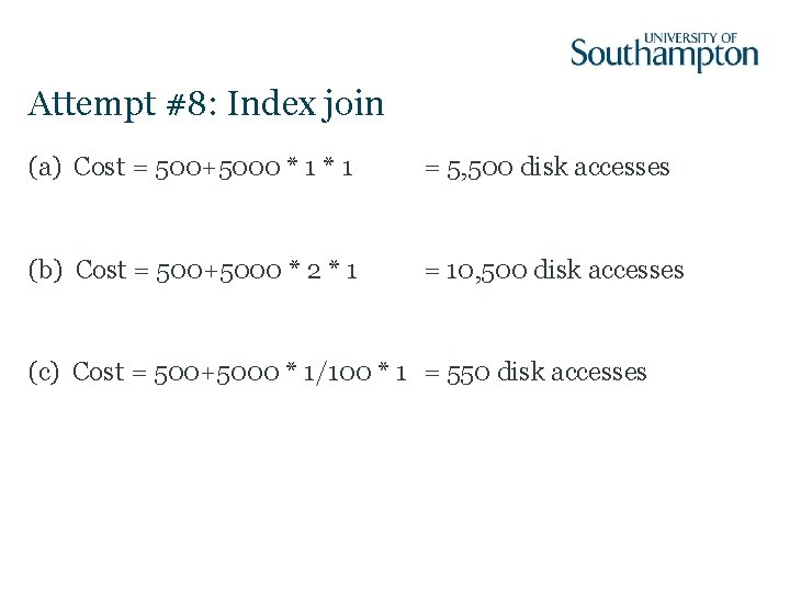
Attempt #8: Index join (a) Cost = 500+5000 * 1 = 5, 500 disk accesses (b) Cost = 500+5000 * 2 * 1 = 10, 500 disk accesses (c) Cost = 500+5000 * 1/100 * 1 = 550 disk accesses

Optimisation
Optimisation A challenge and an opportunity for relational systems – Optimisation must be carried out to achieve performance – Because queries are expressed at such a high semantic level, it is possible for the DBMS to work out the best way to do things Need to start optimisation from a canonical form
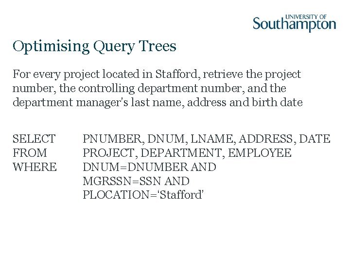
Optimising Query Trees For every project located in Stafford, retrieve the project number, the controlling department number, and the department manager’s last name, address and birth date SELECT FROM WHERE PNUMBER, DNUM, LNAME, ADDRESS, DATE PROJECT, DEPARTMENT, EMPLOYEE DNUM=DNUMBER AND MGRSSN=SSN AND PLOCATION=‘Stafford’
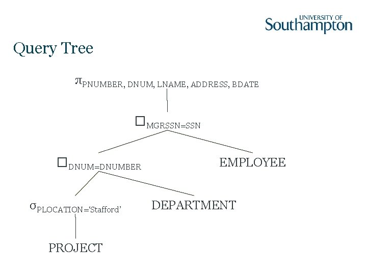
Query Tree πPNUMBER, DNUM, LNAME, ADDRESS, BDATE �MGRSSN=SSN �DNUM=DNUMBER σPLOCATION=‘Stafford’ PROJECT EMPLOYEE DEPARTMENT
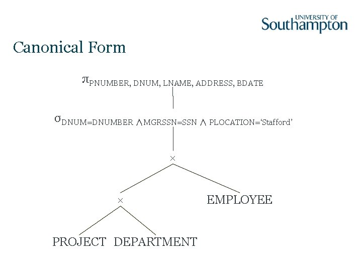
Canonical Form πPNUMBER, DNUM, LNAME, ADDRESS, BDATE σDNUM=DNUMBER ∧MGRSSN=SSN ∧ PLOCATION=‘Stafford’ × × PROJECT DEPARTMENT EMPLOYEE
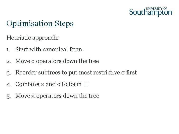
Optimisation Steps Heuristic approach: 1. Start with canonical form 2. Move σ operators down the tree 3. Reorder subtrees to put most restrictive σ first 4. Combine × and σ to form � 5. Move π operators down the tree
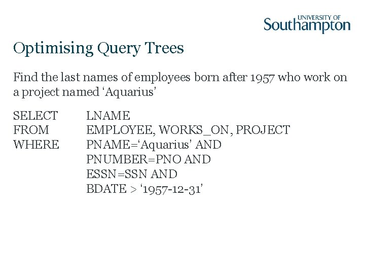
Optimising Query Trees Find the last names of employees born after 1957 who work on a project named ‘Aquarius’ SELECT FROM WHERE LNAME EMPLOYEE, WORKS_ON, PROJECT PNAME=‘Aquarius’ AND PNUMBER=PNO AND ESSN=SSN AND BDATE > ‘ 1957 -12 -31’
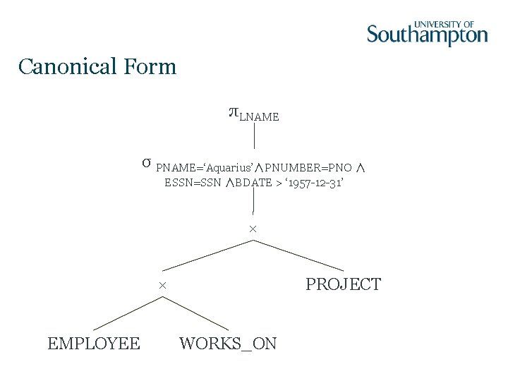
Canonical Form πLNAME σ PNAME=‘Aquarius’∧PNUMBER=PNO ∧ ESSN=SSN ∧BDATE > ‘ 1957 -12 -31’ × × EMPLOYEE PROJECT WORKS_ON
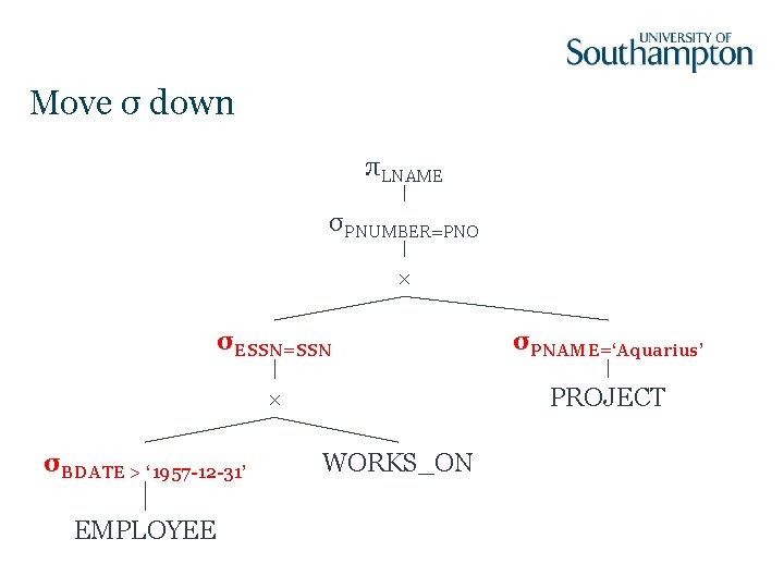
Move σ down πLNAME σPNUMBER=PNO × σESSN=SSN σPNAME=‘Aquarius’ × PROJECT σBDATE > ‘ 1957 -12 -31’ EMPLOYEE WORKS_ON
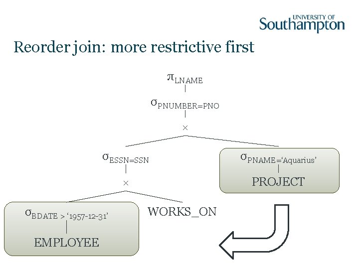
Reorder join: more restrictive first πLNAME σPNUMBER=PNO × σESSN=SSN σPNAME=‘Aquarius’ × PROJECT σBDATE > ‘ 1957 -12 -31’ EMPLOYEE WORKS_ON
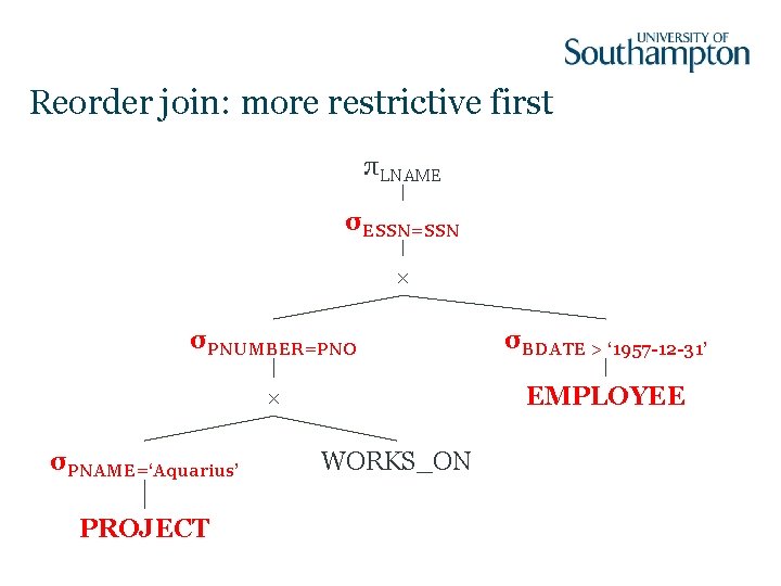
Reorder join: more restrictive first πLNAME σESSN=SSN × σPNUMBER=PNO σBDATE > ‘ 1957 -12 -31’ × EMPLOYEE σPNAME=‘Aquarius’ PROJECT WORKS_ON
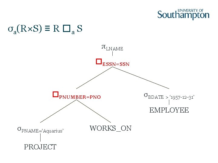
σa(R×S) ≡ R �a S πLNAME �ESSN=SSN �PNUMBER=PNO σBDATE > ‘ 1957 -12 -31’ EMPLOYEE σPNAME=‘Aquarius’ PROJECT WORKS_ON
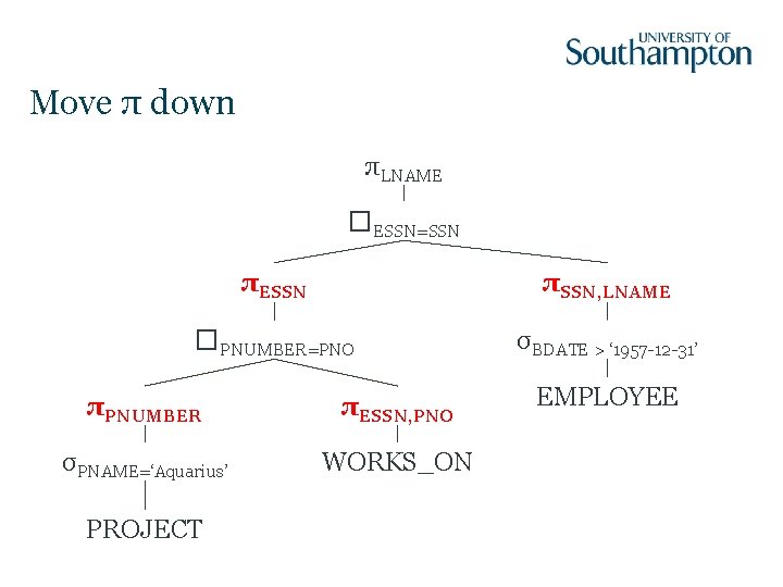
Move π down πLNAME �ESSN=SSN πESSN πSSN, LNAME �PNUMBER=PNO σBDATE > ‘ 1957 -12 -31’ πPNUMBER πESSN, PNO σPNAME=‘Aquarius’ WORKS_ON PROJECT EMPLOYEE
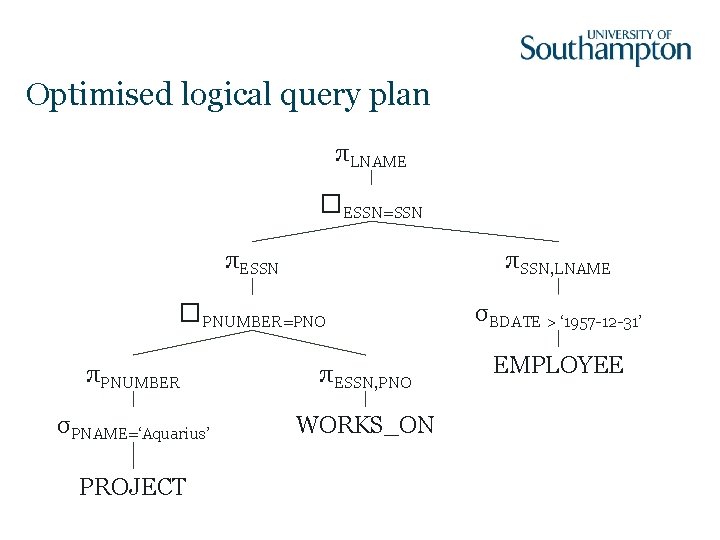
Optimised logical query plan πLNAME �ESSN=SSN πESSN πSSN, LNAME �PNUMBER=PNO σBDATE > ‘ 1957 -12 -31’ πPNUMBER πESSN, PNO σPNAME=‘Aquarius’ WORKS_ON PROJECT EMPLOYEE
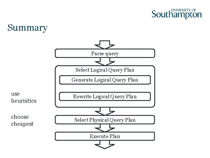
Summary Parse query Select Logical Query Plan Generate Logical Query Plan use heuristics Rewrite Logical Query Plan choose cheapest Select Physical Query Plan Execute Plan
- Slides: 73