QUERY OPTIMIZATION E 0 261 Jayant Haritsa Computer

QUERY OPTIMIZATION E 0 261 Jayant Haritsa Computer Science and Automation Indian Institute of Science AUG 2018 QUERY OPTIMIZATION Slide 1

Database Engines • Main Components – Query Processing – Transaction Processing – Access Methods AUG 2018 QUERY OPTIMIZATION Slide 2

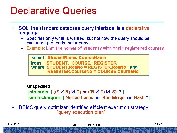
Declarative Queries • SQL, the standard database query interface, is a declarative language – Specifies only what is wanted, but not how the query should be evaluated (i. e. ends, not means) – Example: List the names of students with their registered courses select Student. Name, Course. Name from STUDENT, COURSE, REGISTER where STUDENT. Roll. No = REGISTER. Roll. No and REGISTER. Course. No = COURSE. Course. No Unspecified: join order [ ((S ⨝ R) ⨝ C) or ((R ⨝ C) ⨝ S) ? ] join techniques [ Nested-Loops or Sort-Merge or Hash ? ] • DBMS query optimizer identifies efficient execution strategy: “query execution plan” AUG 2018 QUERY OPTIMIZATION Slide 3

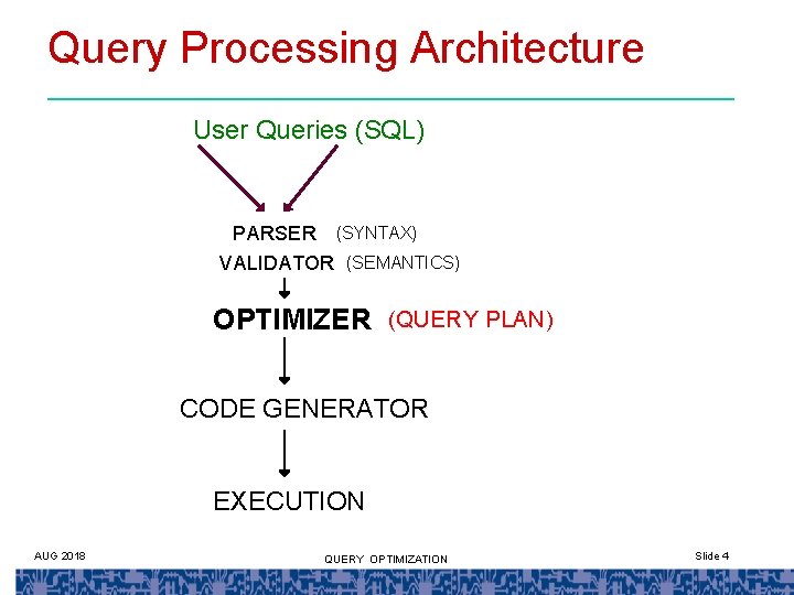
Query Processing Architecture User Queries (SQL) PARSER (SYNTAX) VALIDATOR (SEMANTICS) OPTIMIZER (QUERY PLAN) CODE GENERATOR EXECUTION AUG 2018 QUERY OPTIMIZATION Slide 4

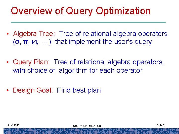
Overview of Query Optimization • Algebra Tree: Tree of relational algebra operators (σ, π, ⨝, …) that implement the user’s query • Query Plan: Tree of relational algebra operators, with choice of algorithm for each operator • Design Goal: Find best plan AUG 2018 QUERY OPTIMIZATION Slide 5

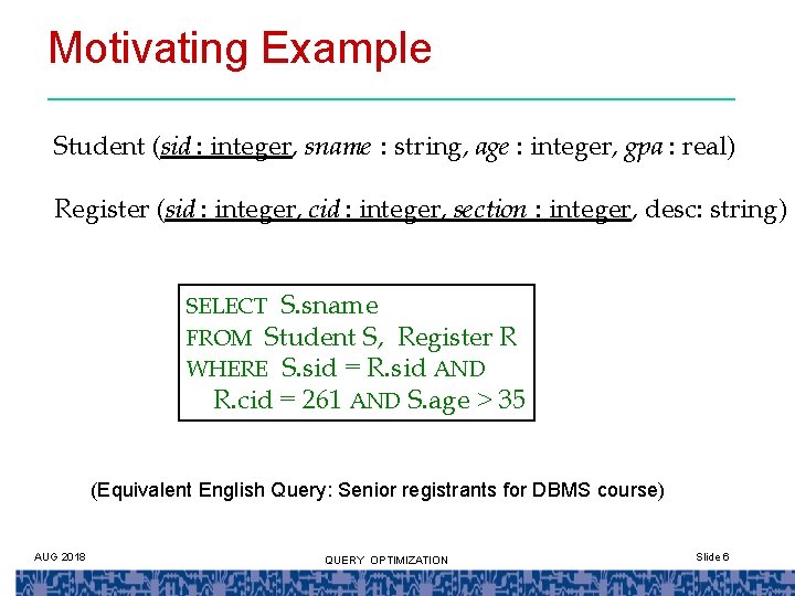
Motivating Example Student (sid : integer, sname : string, age : integer, gpa : real) Register (sid : integer, cid : integer, section : integer, desc: string) SELECT S. sname FROM Student S, Register R WHERE S. sid = R. sid AND R. cid = 261 AND S. age > 35 (Equivalent English Query: Senior registrants for DBMS course) AUG 2018 QUERY OPTIMIZATION Slide 6

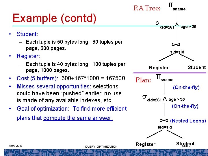
Example (contd) RA Tree: sname cid=261 age > 35 • Student: – Each tuple is 50 bytes long, 80 tuples per page, 500 pages. sid=sid • Register: – Each tuple is 40 bytes long, 100 tuples per page, 1000 pages. • Cost (5 buffers): 500+167*1000 = 167500 • Misses several opportunities: selections could have been “pushed” earlier, no use is made of any available indexes, etc. • Goal of optimization: To find more efficient Student Register Plan: sname (On-the-fly) cid=261 age > 35 (On-the-fly) plans that compute the same answer. (Nested Loops) sid=sid AUG 2018 QUERY OPTIMIZATION Register Student Slide 7

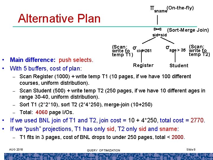
(On-the-fly) sname Alternative Plan sid=sid • Main difference: push selects. • With 5 buffers, cost of plan: – – (Scan; write to cid=261 temp T 1) Register (Sort-Merge Join) (Scan; write to temp T 2) age > 35 Student Scan Register (1000) + write temp T 1 (10 pages, if we have 100 different courses, uniform distribution). Scan Student (500) + write temp T 2 (250 pages, if we have 10 different ages in range 30 -40, uniform distribution). Sort T 1 (2*2*10), sort T 2 (2*4*250), merge-join (10+250) Total: 4060 page I/Os. • If we used BNL join of T 1 and T 2, join cost = 10 + 4*250, total cost = 2770. • If we “push” projections, T 1 has only sid, T 2 only sid and sname: – T 1 fits in 3 pages, cost of BNL drops to under 250 pages, total < 2000. AUG 2018 QUERY OPTIMIZATION Slide 8

Design Framework • Issues – For a given query, what plans are considered (i. e. plan space)? – How is the cost of a plan estimated (i. e. cost model, statistics)? – How to efficiently search through plan space for “cheapest” plan? AUG 2018 QUERY OPTIMIZATION Slide 9

Design Framework (contd) • Ideally: Want to find best plan Practically: Avoid worst plans! • System R approach – 1979 ACM Sigmod conference − paper considered “Bible” of query optimization – Most widely used currently; works well for < 10 joins. P. Selinger, M. Astrahan, D. Chamberlin, R. Lorie and T. Price, “Access Path Selection in a Relational Database System”, Proc. of ACM SIGMOD Intl. Conf. on Management of Data, June 1979. AUG 2018 QUERY OPTIMIZATION Slide 10

Overview of System R Optimizer AUG 2018 QUERY OPTIMIZATION Slide 11

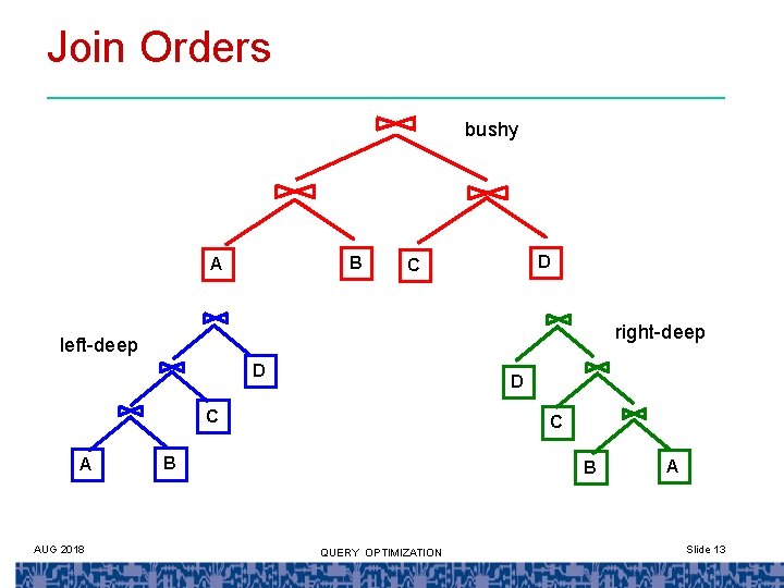
Issue 1: Plan Space • Operator Algorithms: – Access: Sequential, Index (clustered / unclustered) – Join: Nested. Loop, Sort-merge • Plan Structure: – Only left-deep plans are considered • Left-deep plans allow output of each operator to be pipelined into the next operator without storing it in a temporary relation. – Cartesian products are avoided AUG 2018 QUERY OPTIMIZATION Slide 12

Join Orders bushy B A D C right-deep left-deep D D C A AUG 2018 C B B QUERY OPTIMIZATION A Slide 13

Issue 2: Cost Model • Weighted combination of CPU and I/O costs • Simple statistics of relations and indexes maintained in system catalogs • Assume independence across predicates and uniform data distribution across domain • “Wet finger” technique when stats not available! • Statistics are only periodically updated – ensures that metadata locking does not become a bottleneck! AUG 2018 QUERY OPTIMIZATION Slide 14

Issue 3: Search Algorithm • Given an n-relation join, there are n! plans possible (not factoring in choice of join method) • Plan prefixes are “memoryless” about order, therefore use Dynamic Programming (DP) • DP works for n 10 AUG 2018 QUERY OPTIMIZATION Slide 15

Details of System R Optimizer AUG 2018 QUERY OPTIMIZATION Slide 16

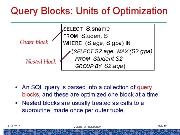
Query Blocks: Units of Optimization Outer block Nested block SELECT S. sname FROM Student S WHERE (S. age, S. gpa) IN (SELECT S 2. age, MAX (S 2. gpa) FROM Student S 2 GROUP BY S 2. age) • An SQL query is parsed into a collection of query blocks, and these are optimized one block at a time. • Nested blocks are usually treated as calls to a subroutine, made once per outer tuple. AUG 2018 QUERY OPTIMIZATION Slide 17

Estimations • For each plan considered: – – AUG 2018 Must estimate cost of each operation in plan tree. Must estimate size of result (cardinality) for each operation in tree. QUERY OPTIMIZATION Slide 18

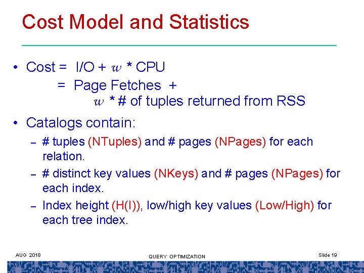
Cost Model and Statistics • Cost = I/O + w * CPU = Page Fetches + w * # of tuples returned from RSS • Catalogs contain: – – – AUG 2018 # tuples (NTuples) and # pages (NPages) for each relation. # distinct key values (NKeys) and # pages (NPages) for each index. Index height (H(I)), low/high key values (Low/High) for each tree index. QUERY OPTIMIZATION Slide 19

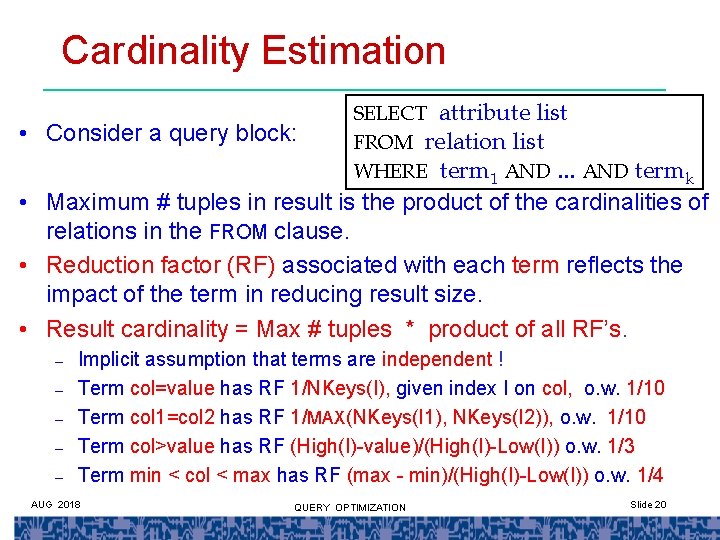
Cardinality Estimation • Consider a query block: SELECT attribute list FROM relation list WHERE term 1 AND. . . AND termk • Maximum # tuples in result is the product of the cardinalities of relations in the FROM clause. • Reduction factor (RF) associated with each term reflects the impact of the term in reducing result size. • Result cardinality = Max # tuples * product of all RF’s. – – – Implicit assumption that terms are independent ! Term col=value has RF 1/NKeys(I), given index I on col, o. w. 1/10 Term col 1=col 2 has RF 1/MAX(NKeys(I 1), NKeys(I 2)), o. w. 1/10 Term col>value has RF (High(I)-value)/(High(I)-Low(I)) o. w. 1/3 Term min < col < max has RF (max - min)/(High(I)-Low(I)) o. w. 1/4 AUG 2018 QUERY OPTIMIZATION Slide 20

Costing Query Blocks • Various cases: – – – AUG 2018 Single-relation query block Multiple-relation query block Nested-query blocks QUERY OPTIMIZATION Slide 21

Single-relation Block • For queries over a single relation, queries consist of a combination of selects, projects, and aggregate ops: – – AUG 2018 Each available access path (file scan / index) is considered, and the one with the least estimated cost is chosen. The different operations are essentially carried out together (e. g. , if an index is used for a selection, projection is done for each retrieved tuple, and the resulting tuples are pipelined into the aggregate computation). QUERY OPTIMIZATION Slide 22

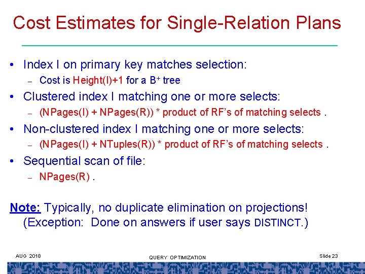
Cost Estimates for Single-Relation Plans • Index I on primary key matches selection: – Cost is Height(I)+1 for a B+ tree • Clustered index I matching one or more selects: – (NPages(I) + NPages(R)) * product of RF’s of matching selects. • Non-clustered index I matching one or more selects: – (NPages(I) + NTuples(R)) * product of RF’s of matching selects. • Sequential scan of file: – NPages(R). Note: Typically, no duplicate elimination on projections! (Exception: Done on answers if user says DISTINCT. ) AUG 2018 QUERY OPTIMIZATION Slide 23

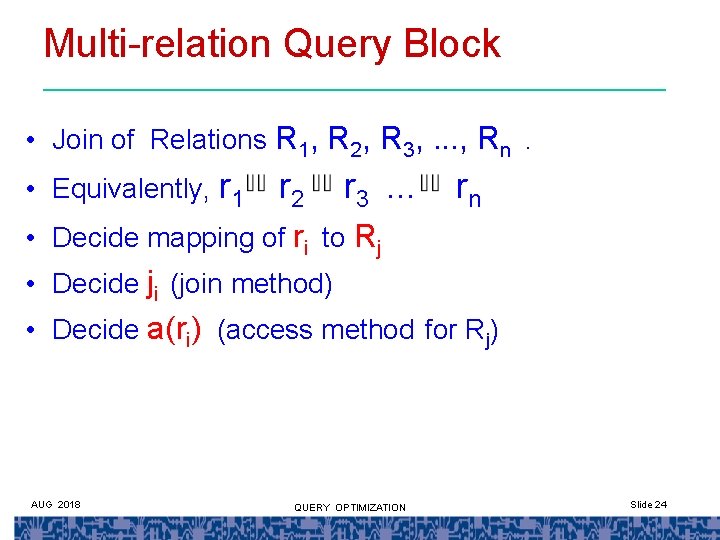
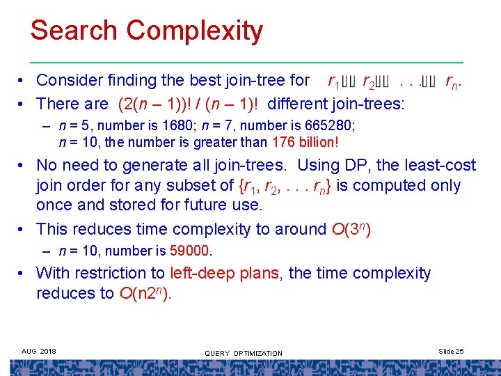
Multi-relation Query Block • Join of Relations R 1, R 2, R 3, . . . , Rn. • Equivalently, r 1 r 2 r 3. . . • Decide mapping of ri to Rj rn • Decide ji (join method) • Decide a(ri) (access method for Rj) AUG 2018 QUERY OPTIMIZATION Slide 24

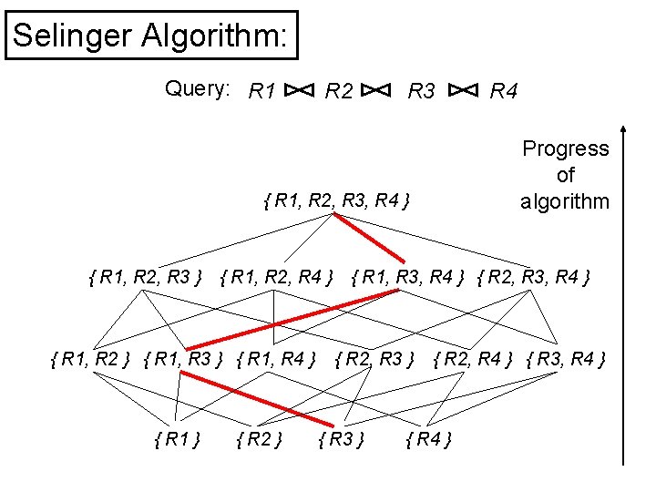
Search Complexity • Consider finding the best join-tree for r 1 r 2. . . • There are (2(n – 1))! / (n – 1)! different join-trees: rn. – n = 5, number is 1680; n = 7, number is 665280; n = 10, the number is greater than 176 billion! • No need to generate all join-trees. Using DP, the least-cost join order for any subset of {r 1, r 2, . . . rn} is computed only once and stored for future use. • This reduces time complexity to around O(3 n) – n = 10, number is 59000. • With restriction to left-deep plans, the time complexity reduces to O(n 2 n). AUG 2018 QUERY OPTIMIZATION Slide 25

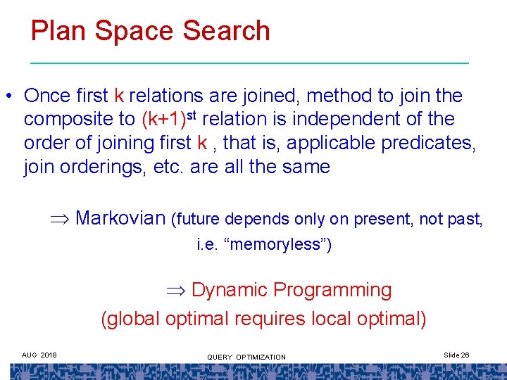
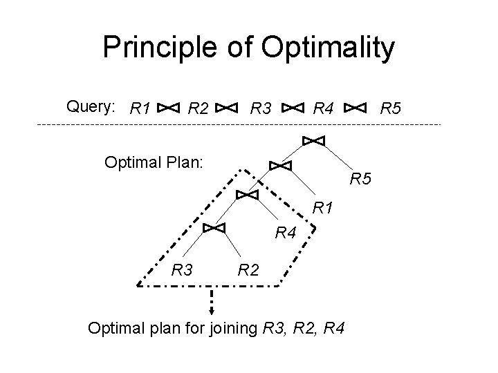
Plan Space Search • Once first k relations are joined, method to join the composite to (k+1)st relation is independent of the order of joining first k , that is, applicable predicates, join orderings, etc. are all the same Markovian (future depends only on present, not past, i. e. “memoryless”) Dynamic Programming (global optimal requires local optimal) AUG 2018 QUERY OPTIMIZATION Slide 26

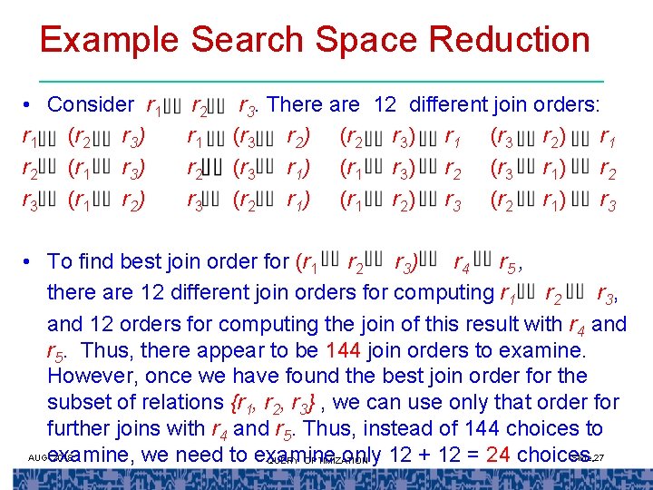
Example Search Space Reduction • Consider r 1 (r 2 r 3) r 2 (r 1 r 3) r 3 (r 1 r 2) r 2 r 1 r 2 r 3. There are 12 different join orders: (r 3 r 2) (r 2 r 3) r 1 (r 3 r 2) r 1 (r 3 r 1) (r 1 r 3) r 2 (r 3 r 1) r 2 (r 2 r 1) (r 1 r 2) r 3 (r 2 r 1) r 3 • To find best join order for (r 1 r 2 r 3) r 4 r 5 , there are 12 different join orders for computing r 1 r 2 r 3, and 12 orders for computing the join of this result with r 4 and r 5. Thus, there appear to be 144 join orders to examine. However, once we have found the best join order for the subset of relations {r 1, r 2, r 3} , we can use only that order for further joins with r 4 and r 5. Thus, instead of 144 choices to Slide 27 AUGexamine, 2018 we need to examine only 12 + 12 = 24 choices. QUERY OPTIMIZATION

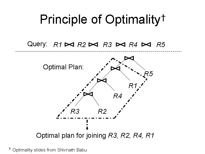
Principle of Optimality† Query: R 1 R 2 R 3 R 4 Optimal Plan: R 5 R 1 R 4 R 3 R 2 Optimal plan for joining R 3, R 2, R 4, R 1 † Optimality slides from Shivnath Babu

Principle of Optimality Query: R 1 R 2 R 3 R 4 Optimal Plan: R 5 R 1 R 4 R 3 R 5 R 2 Optimal plan for joining R 3, R 2, R 4

Selinger Algorithm: Query: R 1 R 2 R 3 Progress of algorithm { R 1, R 2, R 3, R 4 } { R 1, R 2, R 3 } { R 1, R 2, R 4 } { R 1, R 2 } { R 1, R 3 } { R 1, R 4 } { R 1 } { R 2 } R 4 { R 1, R 3, R 4 } { R 2, R 3 } { R 2, R 4 } { R 3, R 4 } { R 4 }

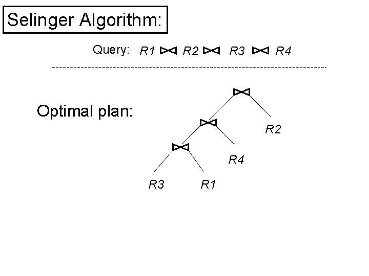
Selinger Algorithm: Query: R 1 R 2 R 3 R 4 Optimal plan: R 2 R 4 R 3 R 1

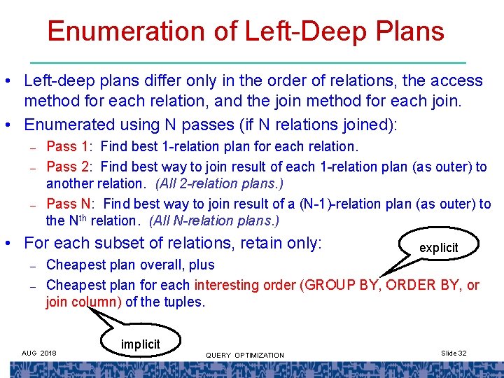
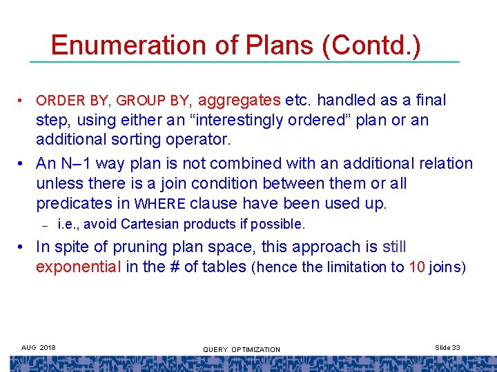
Enumeration of Left-Deep Plans • Left-deep plans differ only in the order of relations, the access method for each relation, and the join method for each join. • Enumerated using N passes (if N relations joined): – – – Pass 1: Find best 1 -relation plan for each relation. Pass 2: Find best way to join result of each 1 -relation plan (as outer) to another relation. (All 2 -relation plans. ) Pass N: Find best way to join result of a (N-1)-relation plan (as outer) to the Nth relation. (All N-relation plans. ) • For each subset of relations, retain only: – – explicit Cheapest plan overall, plus Cheapest plan for each interesting order (GROUP BY, ORDER BY, or join column) of the tuples. AUG 2018 implicit QUERY OPTIMIZATION Slide 32

Enumeration of Plans (Contd. ) • ORDER BY, GROUP BY, aggregates etc. handled as a final step, using either an “interestingly ordered” plan or an additional sorting operator. • An N– 1 way plan is not combined with an additional relation unless there is a join condition between them or all predicates in WHERE clause have been used up. – i. e. , avoid Cartesian products if possible. • In spite of pruning plan space, this approach is still exponential in the # of tables (hence the limitation to 10 joins) AUG 2018 QUERY OPTIMIZATION Slide 33

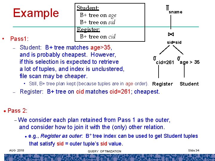
Example Student: B+ tree on age B+ tree on sid Register: B+ tree on cid • Pass 1: – Student: B+ tree matches age>35, and is probably cheapest. However, if this selection is expected to retrieve a lot of tuples, and index is unclustered, file scan may be cheaper. sname sid=sid cid=261 • Still, B+ tree plan kept (because tuples are in age order). Register – · age > 35 Student Register: B+ tree on cid matches cid=261; cheapest. Pass 2: – We consider each plan retained from Pass 1 as the outer, and consider how to join it with the (only) other relation. · AUG 2018 e. g. , Register as outer: B+ tree index can be used to get Student tuples that satisfy sid = outer tuple’s sid value. QUERY OPTIMIZATION Slide 34

Detailed Example • Work through Figures 3, 4, 5, 6 in the paper AUG 2018 QUERY OPTIMIZATION Slide 35

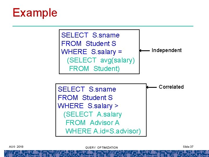
Nested Query Blocks • Uncorrelated nested queries are basically constants to be computed once during execution • Correlated nested queries are like function calls. AUG 2018 QUERY OPTIMIZATION Slide 36

Example SELECT S. sname FROM Student S WHERE S. salary = (SELECT avg(salary) FROM Student) SELECT S. sname FROM Student S WHERE S. salary > (SELECT A. salary FROM Advisor A WHERE A. id=S. advisor) AUG 2018 QUERY OPTIMIZATION Independent Correlated Slide 37

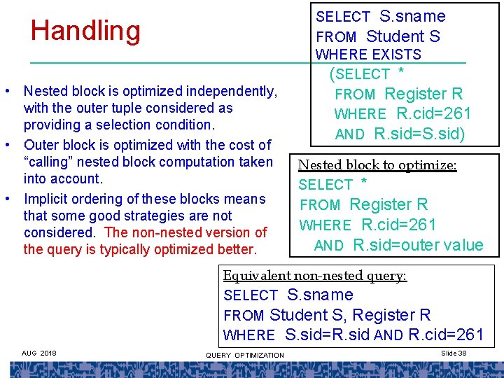
Handling • Nested block is optimized independently, with the outer tuple considered as providing a selection condition. • Outer block is optimized with the cost of “calling” nested block computation taken into account. • Implicit ordering of these blocks means that some good strategies are not considered. The non-nested version of the query is typically optimized better. SELECT S. sname FROM Student S WHERE EXISTS (SELECT * FROM Register R WHERE R. cid=261 AND R. sid=S. sid) Nested block to optimize: SELECT * FROM Register R WHERE R. cid=261 AND R. sid=outer value Equivalent non-nested query: SELECT S. sname FROM Student S, Register R WHERE S. sid=R. sid AND R. cid=261 AUG 2018 QUERY OPTIMIZATION Slide 38

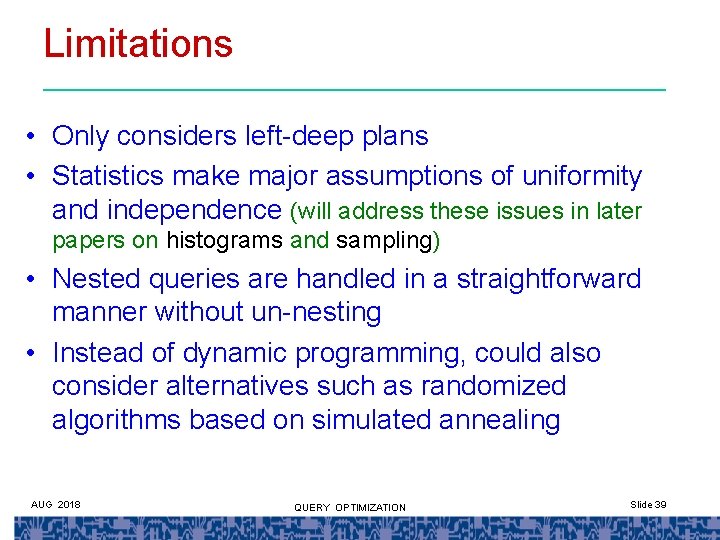
Limitations • Only considers left-deep plans • Statistics make major assumptions of uniformity and independence (will address these issues in later papers on histograms and sampling) • Nested queries are handled in a straightforward manner without un-nesting • Instead of dynamic programming, could also consider alternatives such as randomized algorithms based on simulated annealing AUG 2018 QUERY OPTIMIZATION Slide 39

END QUERY PROCESSING E 0 261 AUG 2018 QUERY OPTIMIZATION Slide 40