Query Evaluation SQL to ERA SQL queries are

Query Evaluation

SQL to ERA • SQL queries are translated into extended relational algebra. • Query evaluation plans are represented as trees of relational operators, with labels identifying the algorithm to use at each node. – Thus, relational operators serve as building blocks for evaluating queries. – Implementation of these operators is carefully optimized for good performance. – Algorithms for individual operators can be combined in many ways to evaluate a query. • The process of finding a good evaluation plan is called query optimization.

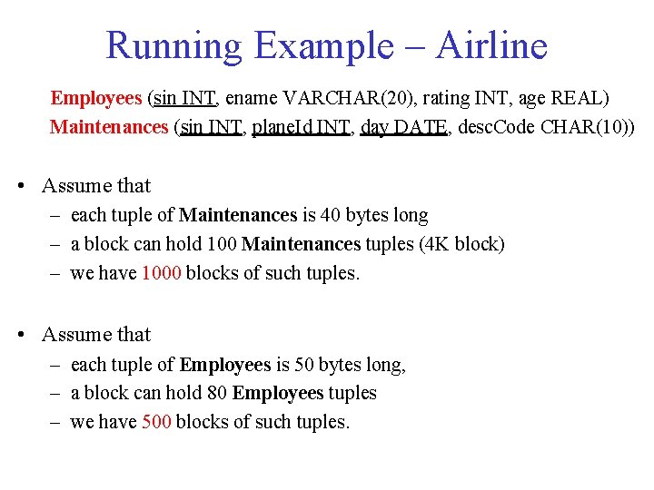
Running Example – Airline Employees (sin INT, ename VARCHAR(20), rating INT, age REAL) Maintenances (sin INT, plane. Id INT, day DATE, desc. Code CHAR(10)) • Assume that – each tuple of Maintenances is 40 bytes long – a block can hold 100 Maintenances tuples (4 K block) – we have 1000 blocks of such tuples. • Assume that – each tuple of Employees is 50 bytes long, – a block can hold 80 Employees tuples – we have 500 blocks of such tuples.

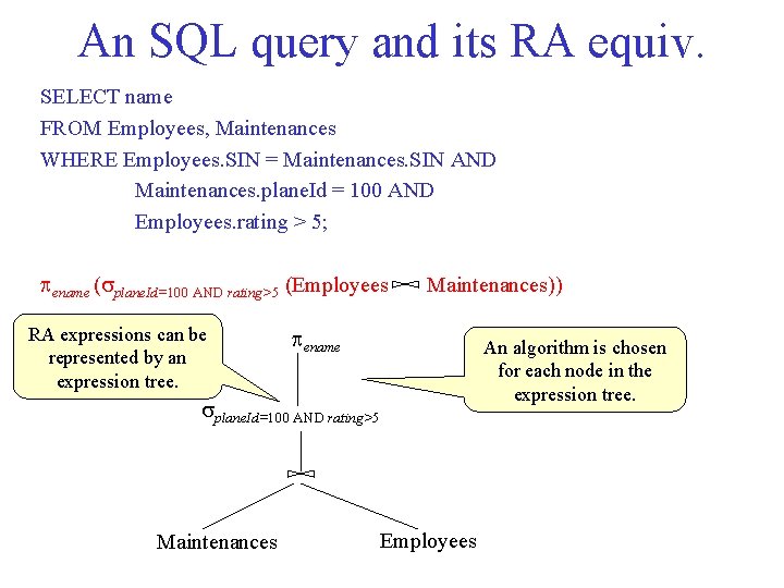
An SQL query and its RA equiv. SELECT name FROM Employees, Maintenances WHERE Employees. SIN = Maintenances. SIN AND Maintenances. plane. Id = 100 AND Employees. rating > 5; ename ( plane. Id=100 AND rating>5 (Employees RA expressions can be represented by an expression tree. Maintenances)) ename An algorithm is chosen for each node in the expression tree. plane. Id=100 AND rating>5 Maintenances Employees

Notions of clustering • Clustered file: e. g. store movie tuples together with the corresponding studio tuple. • Clustered relation: tuples are stored in blocks mostly devoted to that relation. • Clustering index: tuples (of the relation) with same search key are stored together.

Algorithms for selection • Given a selection R. attr = value (R), if there is no index on R. attr, we have to scan R. – How many disk accesses if R is the Maintenances relation? – On average 1000/2 block (pages) reads. • If there is an index we have to typically do 3 disk accesses – This is, assuming a non-clustering B-Tree with 3 levels, with the root in main memory. • Given a selection R. attr < value (R) – Even when there is an non-clustering index we might better scan the relation ignoring the index. Why? – Of course, if we have a clustering index, we use it.

Algorithms for projections • Given a projection we have to scan the relation and drop certain fields of each tuple. – That’s easy. • However, if we need to do a set projection (as opposed to bag projection) specified with the DISTINCT keyword in SQL, we need to remove duplicates. – This is more expensive. – Usually done by sorting, in order to co-locate the duplicates and then remove them. – Can be combined with the final pass of sorting.

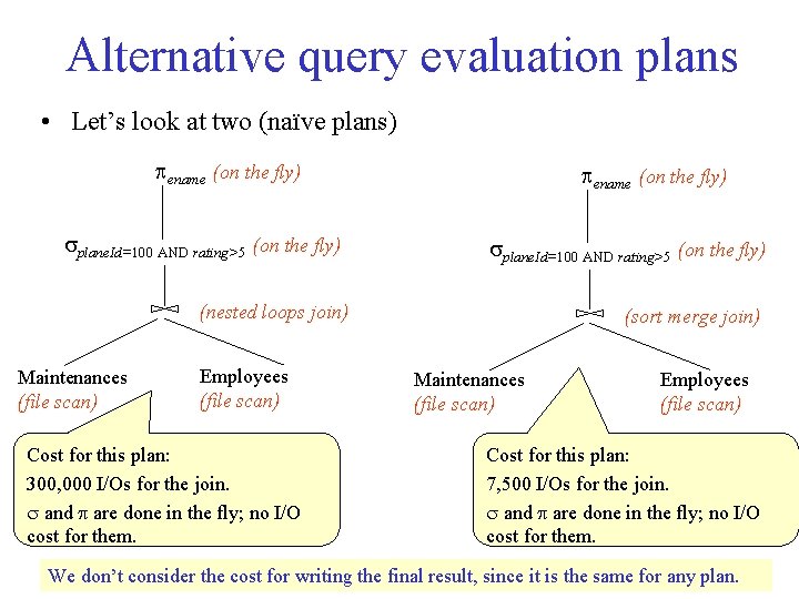
Algorithms for joins • Joins are expensive operations and very common. – They have been widely studied, and systems typically support several algorithms to carry out joins. • Consider the join of Maintenances and Employees, with the join condition Employees. SIN=Maintenance. SIN. • Suppose that one of the tables, say Employees, has an index (BTree) on the sin column. • We can scan Maintenances and, for each tuple, use the index to probe Employees for matching tuples. • This approach is called index nested loops join. • It takes about 3 I/Os on average to retrieve the appropriate page of the index. – For each of the 100, 000 maintenance records we try to access the corresponding employee with 3 I/Os. – So, 100, 000*3 = 300, 000 I/Os on average!!

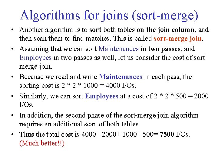
Algorithms for joins (sort-merge) • Another algorithm is to sort both tables on the join column, and then scan them to find matches. This is called sort-merge join. • Assuming that we can sort Maintenances in two passes, and Employees in two passes as well, let us consider the cost of sortmerge join. • Because we read and write Maintenances in each pass, the sorting cost is 2 * 1000 = 4000 I/Os. • Similarly, we can sort Employees at a cost of 2 * 500 = 2000 I/Os. • In addition, the second phase of the sort-merge join algorithm requires an additional scan of both tables. • Thus the total cost is 4000+ 2000+ 1000+ 500= 7500 I/Os. (Much better!!)

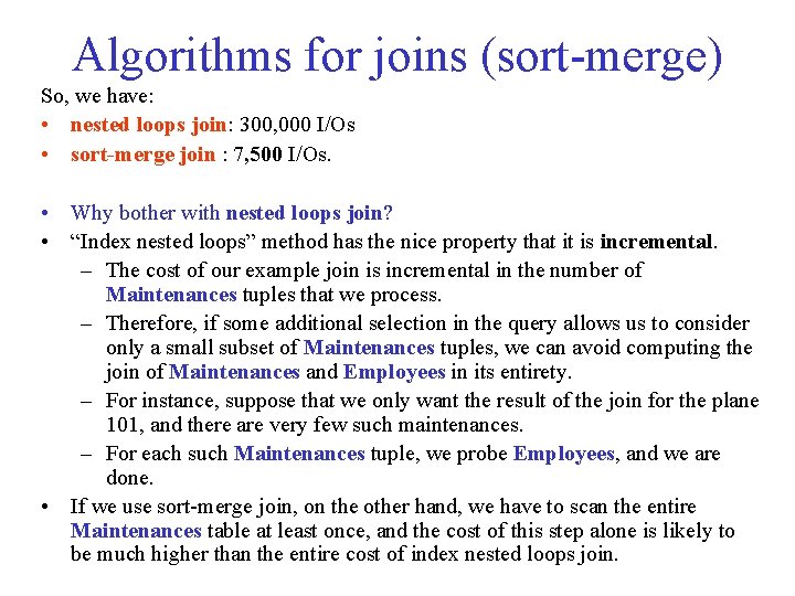
Algorithms for joins (sort-merge) So, we have: • nested loops join: 300, 000 I/Os • sort-merge join : 7, 500 I/Os. • Why bother with nested loops join? • “Index nested loops” method has the nice property that it is incremental. – The cost of our example join is incremental in the number of Maintenances tuples that we process. – Therefore, if some additional selection in the query allows us to consider only a small subset of Maintenances tuples, we can avoid computing the join of Maintenances and Employees in its entirety. – For instance, suppose that we only want the result of the join for the plane 101, and there are very few such maintenances. – For each such Maintenances tuple, we probe Employees, and we are done. • If we use sort-merge join, on the other hand, we have to scan the entire Maintenances table at least once, and the cost of this step alone is likely to be much higher than the entire cost of index nested loops join.

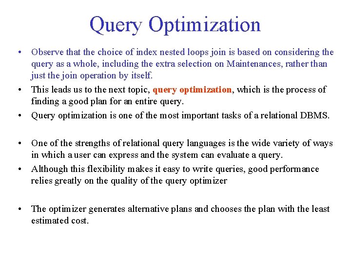
Query Optimization • Observe that the choice of index nested loops join is based on considering the query as a whole, including the extra selection on Maintenances, rather than just the join operation by itself. • This leads us to the next topic, query optimization, which is the process of finding a good plan for an entire query. • Query optimization is one of the most important tasks of a relational DBMS. • One of the strengths of relational query languages is the wide variety of ways in which a user can express and the system can evaluate a query. • Although this flexibility makes it easy to write queries, good performance relies greatly on the quality of the query optimizer • The optimizer generates alternative plans and chooses the plan with the least estimated cost.

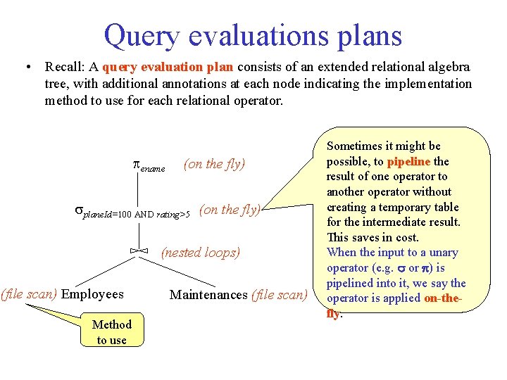
Query evaluations plans • Recall: A query evaluation plan consists of an extended relational algebra tree, with additional annotations at each node indicating the implementation method to use for each relational operator. ename (on the fly) plane. Id=100 AND rating>5 (on the fly) (nested loops) (file scan) Employees Method to use Maintenances (file scan) Sometimes it might be possible, to pipeline the result of one operator to another operator without creating a temporary table for the intermediate result. This saves in cost. When the input to a unary operator (e. g. or ) is pipelined into it, we say the operator is applied on-thefly.

Alternative query evaluation plans • Let’s look at two (naïve plans) ename (on the fly) plane. Id=100 AND rating>5 (on the fly) (nested loops join) Maintenances (file scan) Employees (file scan) Cost for this plan: 300, 000 I/Os for the join. and are done in the fly; no I/O cost for them. (sort merge join) Maintenances (file scan) Employees (file scan) Cost for this plan: 7, 500 I/Os for the join. and are done in the fly; no I/O cost for them. We don’t consider the cost for writing the final result, since it is the same for any plan.

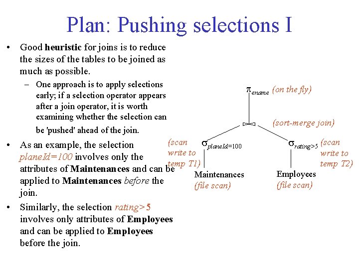
Plan: Pushing selections I • Good heuristic for joins is to reduce the sizes of the tables to be joined as much as possible. – One approach is to apply selections early; if a selection operator appears after a join operator, it is worth examining whether the selection can be 'pushed' ahead of the join. (scan plane. Id=100 • As an example, the selection write to plane. Id=100 involves only the temp T 1) attributes of Maintenances and can be Maintenances applied to Maintenances before the (file scan) join. • Similarly, the selection rating>5 involves only attributes of Employees and can be applied to Employees before the join. ename (on the fly) (sort-merge join) rating>5 (scan write to temp T 2) Employees (file scan)

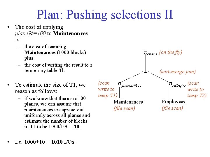
Plan: Pushing selections II • The cost of applying plane. Id=100 to Maintenances is: – the cost of scanning Maintenances (1000 blocks) plus – the cost of writing the result to a temporary table Tl. • To estimate the size of T 1, we reason as follows: – if we know that there are 100 planes, we can assume that maintenances are spread out uniformly across all planes and estimate the number of blocks in T 1 to be 1000/100 = 10. • I. e. 1000+10 = 1010 I/Os. ename (on the fly) (sort-merge join) (scan plane. Id=100 write to temp T 1) Maintenances (file scan) rating>5 (scan write to temp T 2) Employees (file scan)

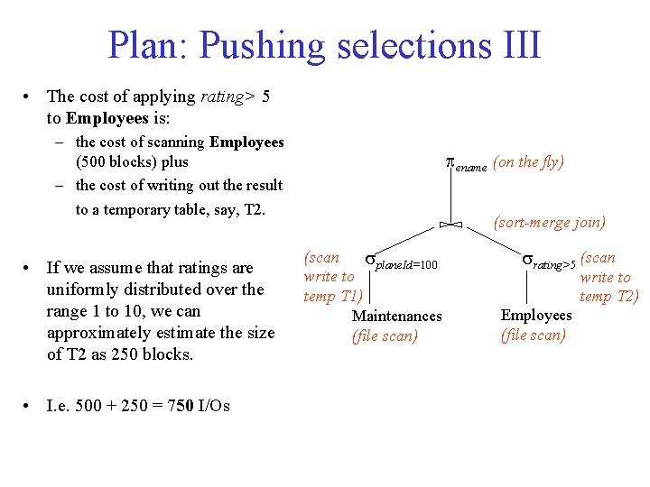
Plan: Pushing selections III • The cost of applying rating> 5 to Employees is: – the cost of scanning Employees (500 blocks) plus – the cost of writing out the result to a temporary table, say, T 2. • If we assume that ratings are uniformly distributed over the range 1 to 10, we can approximately estimate the size of T 2 as 250 blocks. • I. e. 500 + 250 = 750 I/Os ename (on the fly) (sort-merge join) (scan plane. Id=100 write to temp T 1) Maintenances (file scan) rating>5 (scan write to temp T 2) Employees (file scan)

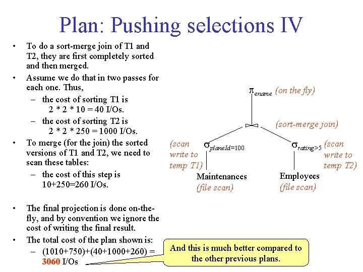
Plan: Pushing selections IV • • • To do a sort-merge join of T 1 and T 2, they are first completely sorted and then merged. Assume we do that in two passes for each one. Thus, – the cost of sorting T 1 is 2 * 10 = 40 I/Os. – the cost of sorting T 2 is 2 * 250 = 1000 I/Os. To merge (for the join) the sorted versions of T 1 and T 2, we need to scan these tables: – the cost of this step is 10+250=260 I/Os. (scan plane. Id=100 write to temp T 1) Maintenances (file scan) The final projection is done on-thefly, and by convention we ignore the cost of writing the final result. The total cost of the plan shown is: – (1010+750)+(40+1000+260) = 3060 I/Os And this is much better compared to the other previous plans. ename (on the fly) (sort-merge join) rating>5 (scan write to temp T 2) Employees (file scan)

Pushing projections • A further refinement is to push the projection, just like we pushed the selections past the join. • Observe that only the SIN attribute of T 1 and the SIN and ename attributes of T 2 are really required. • When we scan Maintenances and Employees to do the selections, we could also eliminate unwanted columns. – This on-the-fly projection reduces the sizes of the temporary tables T 1 and T 2. – The reduction in the size of T 1 is substantial because only an integer field is retained. – In fact, T 1 now fits within three blocks (and be all can be in MM), and we can perform a block nested loops join with a single scan of T 2. – The cost of the join step drops to under 250 page I/Os, and the total cost of the plan drops to about 2000 I/Os.

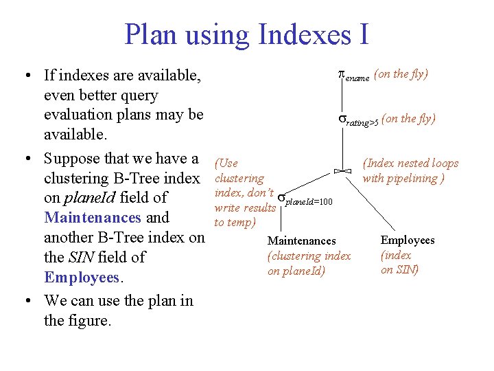
Plan using Indexes I • If indexes are available, even better query evaluation plans may be available. • Suppose that we have a clustering B-Tree index on plane. Id field of Maintenances and another B-Tree index on the SIN field of Employees. • We can use the plan in the figure. ename (on the fly) rating>5 (on the fly) (Use clustering index, don’t plane. Id=100 write results to temp) Maintenances (clustering index on plane. Id) (Index nested loops with pipelining ) Employees (index on SIN)

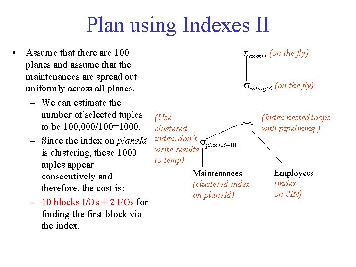
Plan using Indexes II • Assume that there are 100 planes and assume that the maintenances are spread out uniformly across all planes. – We can estimate the number of selected tuples to be 100, 000/100=1000. – Since the index on plane. Id is clustering, these 1000 tuples appear consecutively and therefore, the cost is: – 10 blocks I/Os + 2 I/Os for finding the first block via the index. ename (on the fly) rating>5 (on the fly) (Use clustered index, don’t plane. Id=100 write results to temp) Maintenances (clustered index on plane. Id) (Index nested loops with pipelining ) Employees (index on SIN)

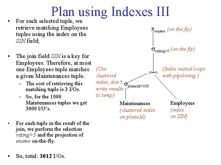
Plan using Indexes III • For each selected tuple, we retrieve matching Employees tuples using the index on the SIN field; ename (on the fly) • The join field SIN is a key for Employees. Therefore, at most one Employees tuple matches (Use clustered a given Maintenances tuple. – The cost of retrieving this matching tuple is 3 I/Os. – So, for the 1000 Maintenances tuples we get 3000 I/O’s. • For each tuple in the result of the join, we perform the selection rating>5 and the projection of ename on-the-fly. • So, total: 3012 I/Os. rating>5 (on the fly) (Index nested loops with pipelining ) index, don’t plane. Id=100 write results to temp) Maintenances (clustered index on plane. Id) Employees (index on SIN)

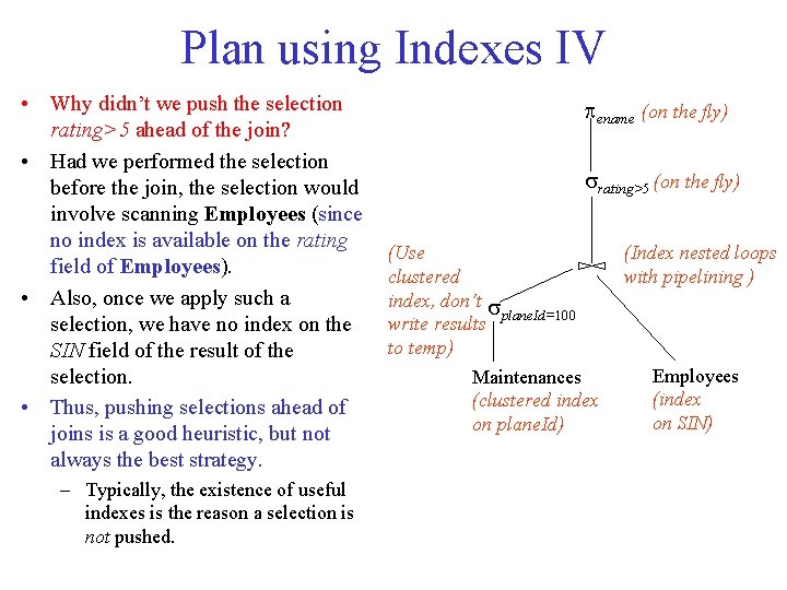
Plan using Indexes IV • Why didn’t we push the selection rating>5 ahead of the join? • Had we performed the selection before the join, the selection would involve scanning Employees (since no index is available on the rating field of Employees). • Also, once we apply such a selection, we have no index on the SIN field of the result of the selection. • Thus, pushing selections ahead of joins is a good heuristic, but not always the best strategy. – Typically, the existence of useful indexes is the reason a selection is not pushed. ename (on the fly) rating>5 (on the fly) (Use clustered index, don’t plane. Id=100 write results to temp) Maintenances (clustered index on plane. Id) (Index nested loops with pipelining ) Employees (index on SIN)

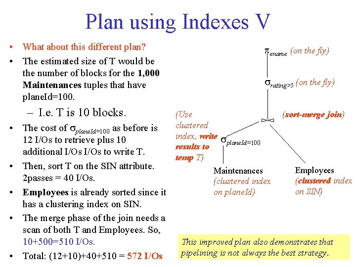
Plan using Indexes V • What about this different plan? • The estimated size of T would be the number of blocks for the 1, 000 Maintenances tuples that have plane. Id=100. – I. e. T is 10 blocks. • The cost of plane. Id=100 as before is 12 I/Os to retrieve plus 10 additional I/Os to write T. • Then, sort T on the SIN attribute. 2 passes = 40 I/Os. • Employees is already sorted since it has a clustering index on SIN. • The merge phase of the join needs a scan of both T and Employees. So, 10+500=510 I/Os. • Total: (12+10)+40+510 = 572 I/Os ename (on the fly) rating>5 (on the fly) (Use clustered index, write plane. Id=100 results to temp T) Maintenances (clustered index on plane. Id) (sort-merge join) Employees (clustered index on SIN) This improved plan also demonstrates that pipelining is not always the best strategy.