Quantum random walks new method for designing quantum

Quantum random walks – new method for designing quantum algorithms Andris Ambainis University of Latvia

Quantum computing n n New model of computing, based on quantum mechanics. More powerful than conventional (classical) computing.

Talk outline 1. 2. 3. Main results of quantum computing. The model. Quantum algorithms based on quantum walks.

Shor’s algorithm n n Factoring: given N=pq, find p and q. 1/3) O(n Best algorithm - 2 , n – number of digits. Quantum algorithm - O(n 3) [Shor, 94]. Cryptosystems based on hardness of factoring/discrete log become insecure.

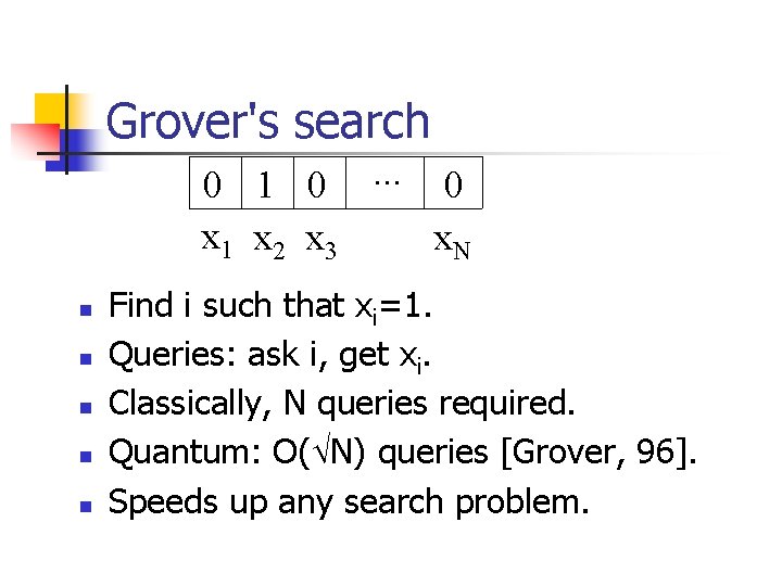
Grover's search 0 1 0. . . 0 x 1 x 2 x 3 x. N n n n Find i such that xi=1. Queries: ask i, get xi. Classically, N queries required. Quantum: O( N) queries [Grover, 96]. Speeds up any search problem.

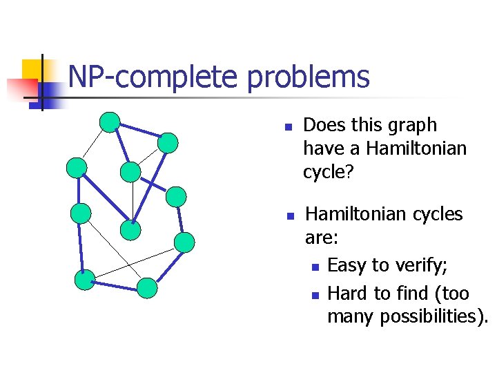
NP-complete problems n n Does this graph have a Hamiltonian cycle? Hamiltonian cycles are: n Easy to verify; n Hard to find (too many possibilities).

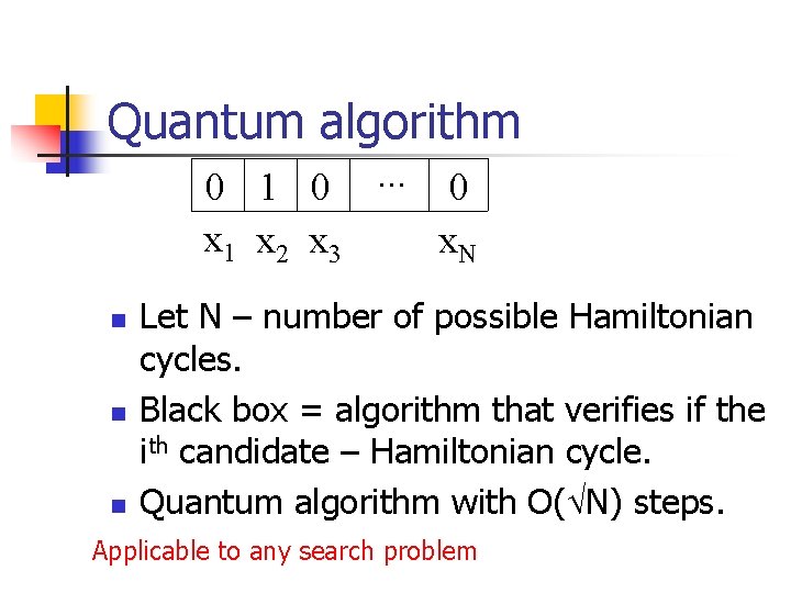
Quantum algorithm 0 1 0. . . 0 x 1 x 2 x 3 x. N n n n Let N – number of possible Hamiltonian cycles. Black box = algorithm that verifies if the ith candidate – Hamiltonian cycle. Quantum algorithm with O( N) steps. Applicable to any search problem

Pell’s equation n Given d, find the smallest solution (x, y) to x 2 -dy 2=1. Probably harder than factoring and discrete logarithm. Best classical algorithms: n n 2 O( N) for factoring; for discrete logarithm. Hallgren, 2001: Quantum algorithm for Pell’s equation.

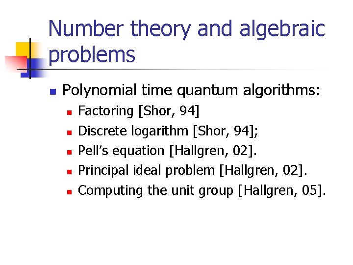
Number theory and algebraic problems n Polynomial time quantum algorithms: n n n Factoring [Shor, 94] Discrete logarithm [Shor, 94]; Pell’s equation [Hallgren, 02]. Principal ideal problem [Hallgren, 02]. Computing the unit group [Hallgren, 05].

Grover's search 0 1 0. . . 0 x 1 x 2 x 3 x. N n n n Find i such that xi=1. Queries: ask i, get xi. Classically, N queries required. Quantum: O( N) queries [Grover, 96]. Speeds up any search problem.

Amplitude amplification [Brassard et al. , 01] n n n Algorithm A that finds a certain object with probability . How many repetitions to achieve probability 2/3? Classically, (1/ ). Quantum: O(1/ ). “Quantum black box”.

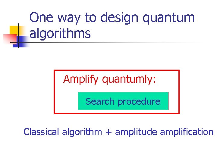
One way to design quantum algorithms Amplify quantumly: Search procedure Classical algorithm + amplitude amplification

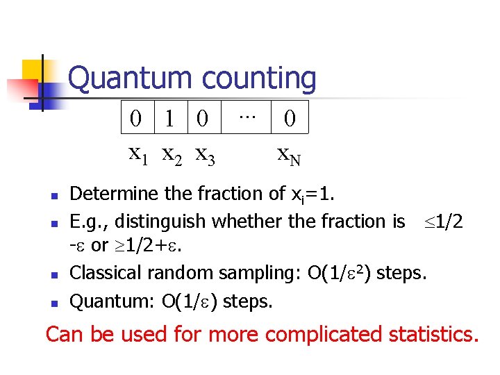
Quantum counting 0 1 0. . . 0 x 1 x 2 x 3 x. N n n Determine the fraction of xi=1. E. g. , distinguish whether the fraction is 1/2 - or 1/2+. Classical random sampling: O(1/ 2) steps. Quantum: O(1/ ) steps. Can be used for more complicated statistics.

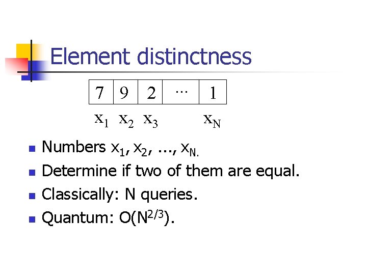
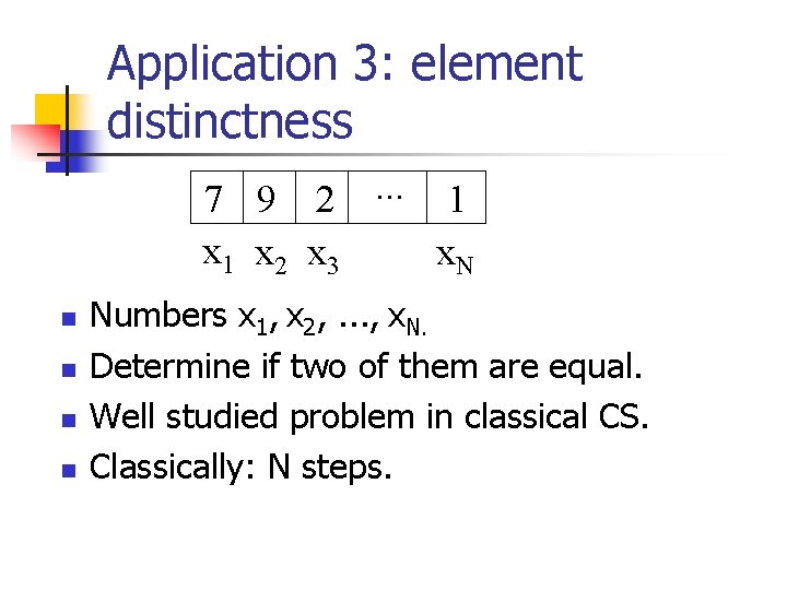
Element distinctness 7 9 2. . . 1 x 2 x 3 x. N n n Numbers x 1, x 2, . . . , x. N. Determine if two of them are equal. Classically: N queries. Quantum: O(N 2/3).

Triangle finding [Magniez, Santha, Szegedy, 03] n n n Graph G with n vertices. n 2 variables xij; xij=1 if there is an edge (i, j). Does G contain a triangle? Classically: O(n 2). Quantum: O(n 1. 3).

The model of quantum computing

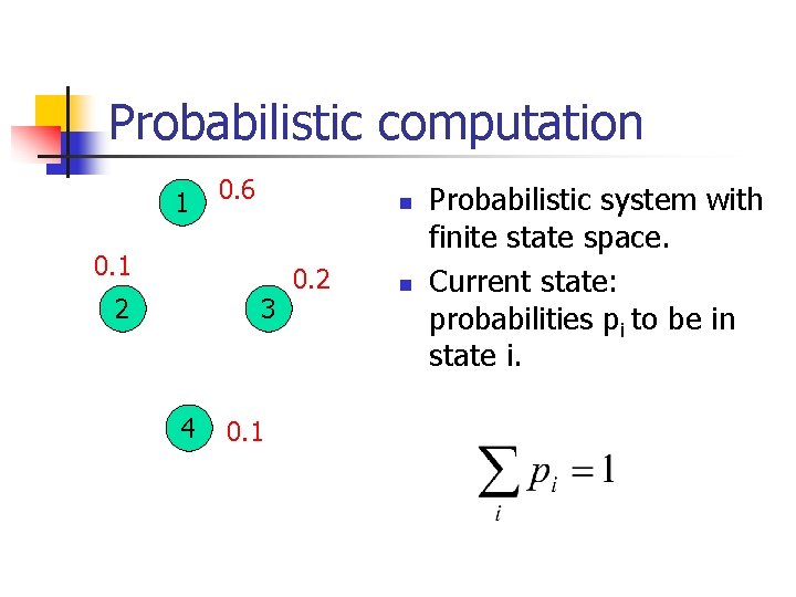
Probabilistic computation 1 0. 6 n 0. 1 2 3 4 0. 1 0. 2 n Probabilistic system with finite state space. Current state: probabilities pi to be in state i.

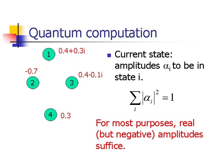
Quantum computation 1 0. 4+0. 3 i -0. 7 2 3 4 0. 3 n 0. 4 -0. 1 i Current state: amplitudes i to be in state i. For most purposes, real (but negative) amplitudes suffice.

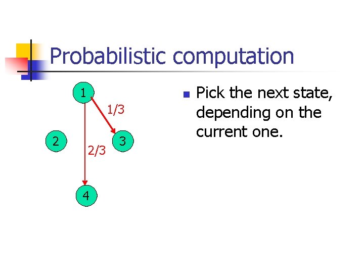
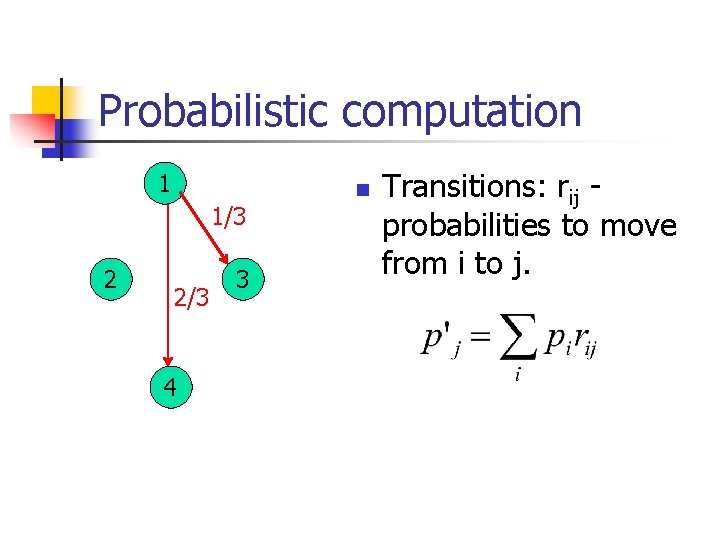
Probabilistic computation 1 n 1/3 2 2/3 4 3 Pick the next state, depending on the current one.

Probabilistic computation 1 1/3 2 2/3 4 3 n Transitions: rij probabilities to move from i to j.

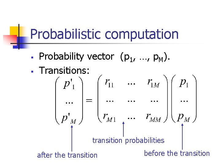
Probabilistic computation § § Probability vector (p 1, …, p. M). Transitions: transition probabilities after the transition before the transition

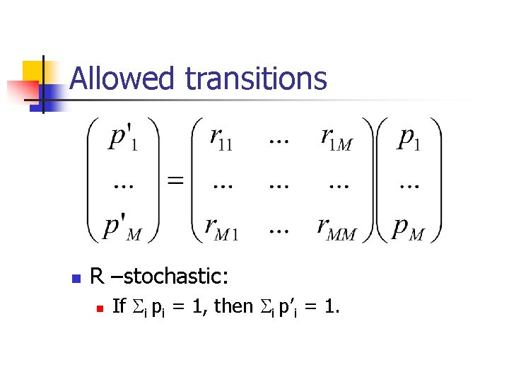
Allowed transitions n R –stochastic: n If i pi = 1, then i p’i = 1.

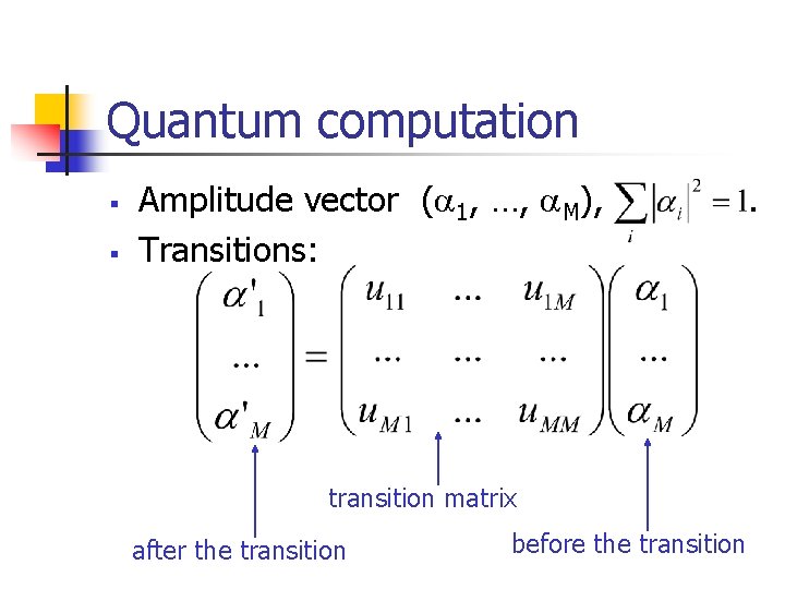
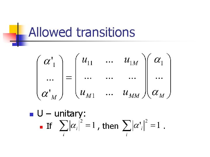
Quantum computation § § Amplitude vector ( 1, …, M), Transitions: transition matrix after the transition before the transition .

Allowed transitions n U – unitary: n If , then .

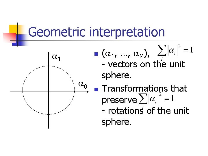
Geometric interpretation 1 n 0 n ( 1, …, M), - vectors on the unit sphere. Transformations that preserve - rotations of the unit sphere.

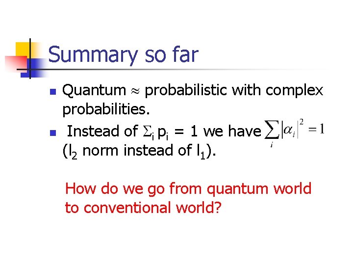
Summary so far n n Quantum probabilistic with complex probabilities. Instead of i pi = 1 we have (l 2 norm instead of l 1). How do we go from quantum world to conventional world?

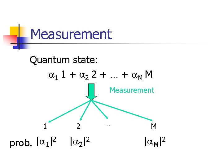
Measurement Quantum state: 1 1 + 2 2 + … + M M Measurement 1 2 | | prob. 1 2 | 2|2 … M | M|2

Quantum walks and quantum algorithms 1. 2. 3. Quantum random walks. Grover’s quantum search algorithm. Quantum walks + quantum algorithms.

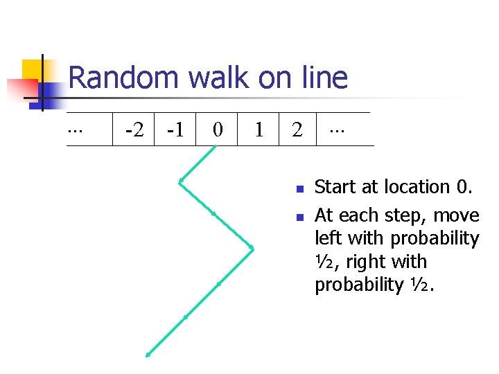
Random walk on line. . . -2 -1 0 1 2 n n . . . Start at location 0. At each step, move left with probability ½, right with probability ½.

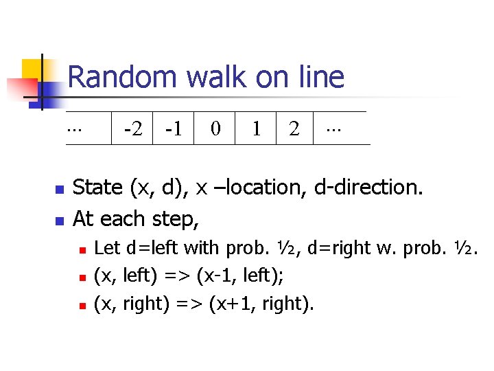
Random walk on line. . . n n -2 -1 0 1 2 . . . State (x, d), x –location, d-direction. At each step, n n n Let d=left with prob. ½, d=right w. prob. ½. (x, left) => (x-1, left); (x, right) => (x+1, right).

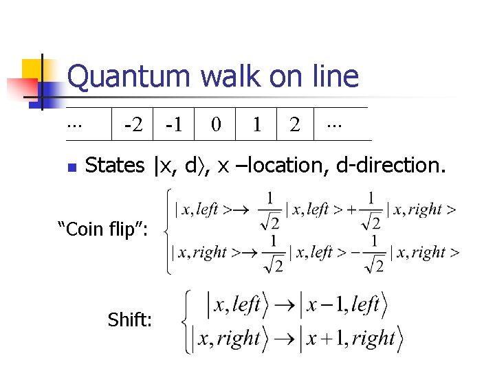
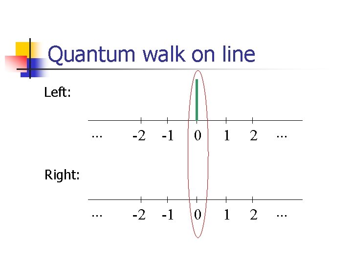
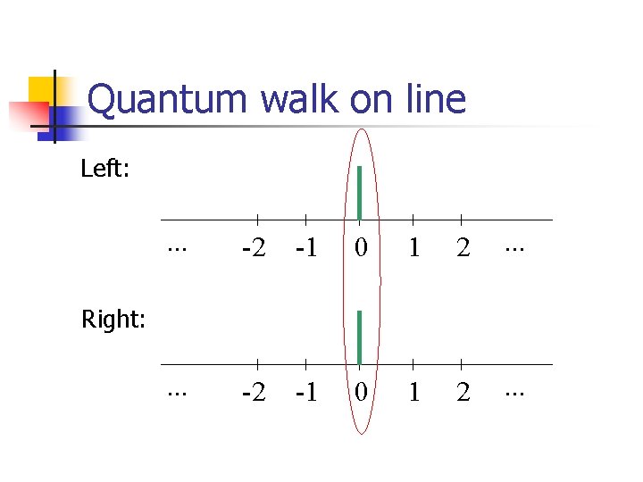
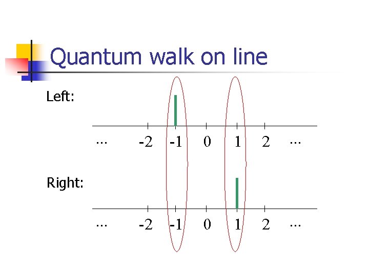
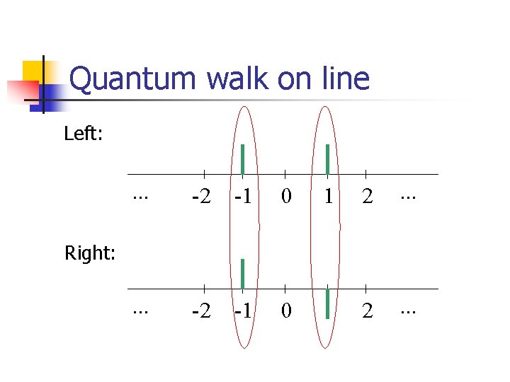
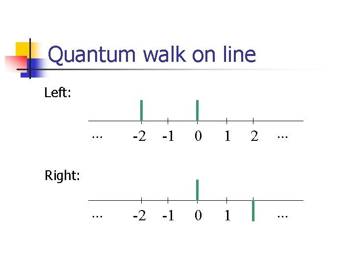
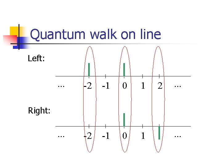
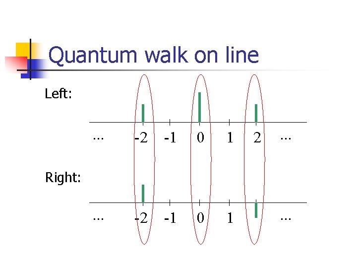
Quantum walk on line. . . n -2 -1 0 1 2 . . . States |x, d , x –location, d-direction. “Coin flip”: Shift:

Quantum walk on line Left: . . . -2 -1 0 1 2 . . . Right:

Quantum walk on line Left: . . . -2 -1 0 1 2 . . . Right:

Quantum walk on line Left: . . . -2 -1 0 1 2 . . . Right:

Quantum walk on line Left: . . . -2 -1 0 1 2 . . . Right:

Quantum walk on line Left: . . . -2 -1 0 1 2 . . . Right: . . .

Quantum walk on line Left: . . . -2 -1 0 1 2 . . . Right: . . .

Quantum walk on line Left: . . . -2 -1 0 1 2 . . . Right: . . .

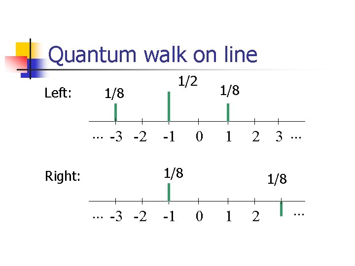
Quantum walk on line Left: 1/2 1/8 . . . -3 -2 -1 0 1/8 1 2 1/8 Right: . . . -3 -2 -1 3. . . 1/8 0 1 2 . . .

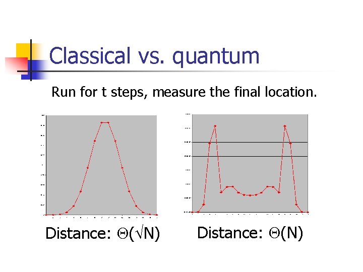
Classical vs. quantum Run for t steps, measure the final location. Distance: ( N) Distance: (N)

Grover’s quantum search algorithm

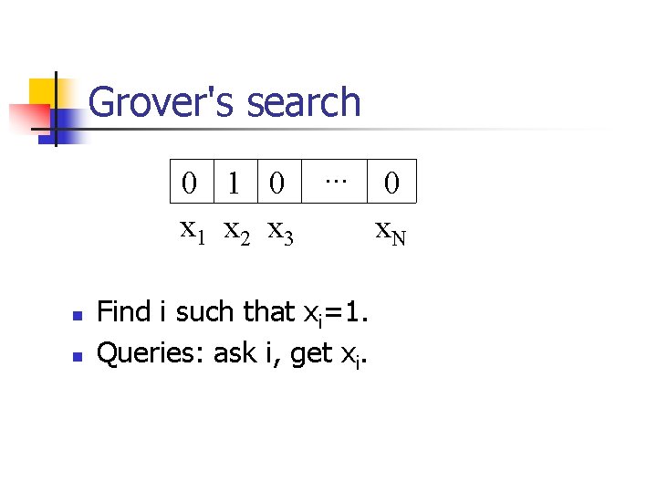
Grover's search 0 1 0. . . 0 x 1 x 2 x 3 x. N n n Find i such that xi=1. Queries: ask i, get xi.

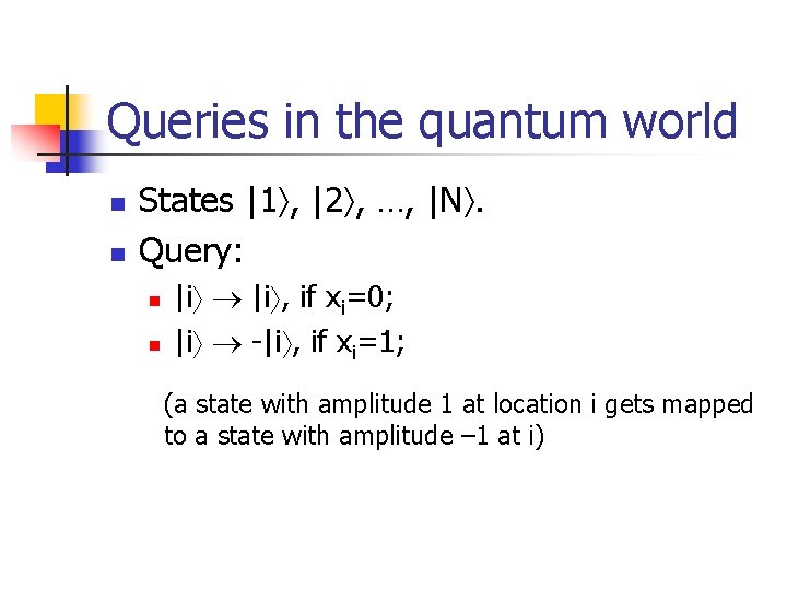
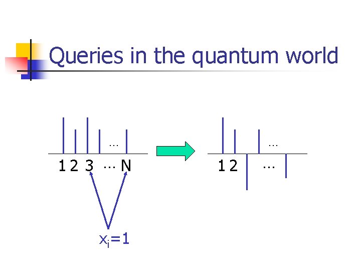
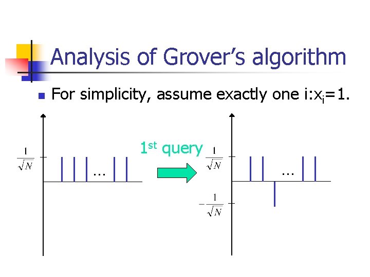
Queries in the quantum world n n States |1 , |2 , …, |N. Query: n n |i , if xi=0; |i -|i , if xi=1; (a state with amplitude 1 at location i gets mapped to a state with amplitude – 1 at i)

Queries in the quantum world … 12 3 … N xi=1 … 12 …

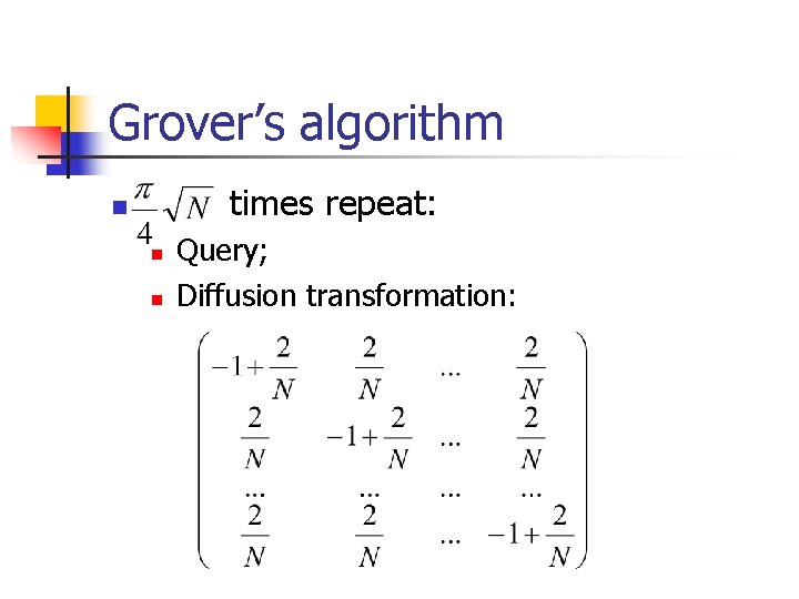
Grover’s algorithm times repeat: n n n Query; Diffusion transformation:

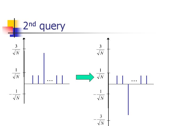
Analysis of Grover’s algorithm n For simplicity, assume exactly one i: xi=1. 1 st query … …

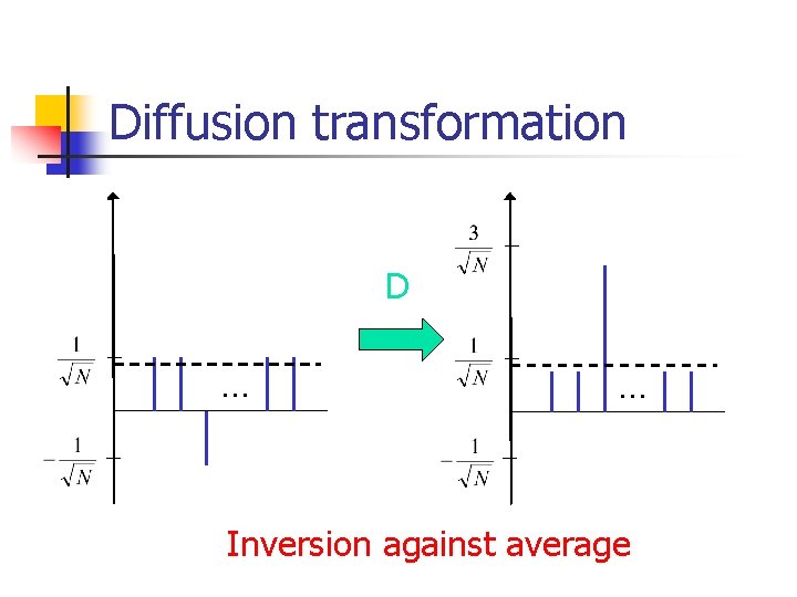
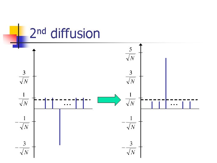
Diffusion transformation D … … Inversion against average

2 nd query … …

2 nd diffusion … …

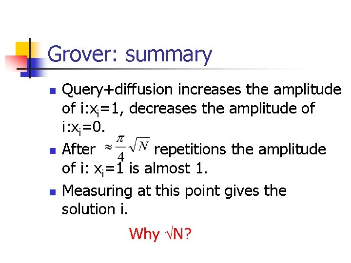
Grover: summary n n n Query+diffusion increases the amplitude of i: xi=1, decreases the amplitude of i: xi=0. After repetitions the amplitude of i: xi=1 is almost 1. Measuring at this point gives the solution i. Why N?

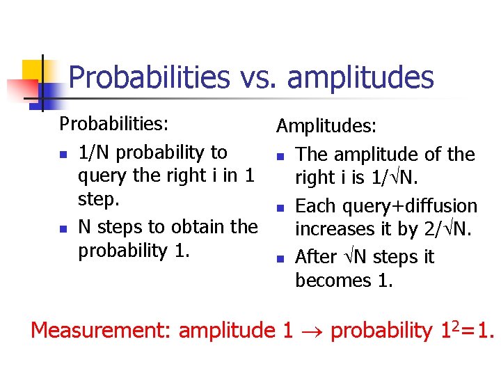
Probabilities vs. amplitudes Probabilities: Amplitudes: n 1/N probability to n The amplitude of the query the right i in 1 right i is 1/ N. step. n Each query+diffusion n N steps to obtain the increases it by 2/ N. probability 1. n After N steps it becomes 1. Measurement: amplitude 1 probability 12=1.

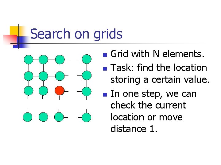
Search on grids n n n Grid with N elements. Task: find the location storing a certain value. In one step, we can check the current location or move distance 1.

[Benioff, 2000] n n n n* n grid. Distance between opposite corners = 2 n. Grover’s algorithm takes steps. n No quantum speedup. Quantum walks solve this problem!

Quantum walk search [Szegedy, 04] 1 n 3 2 n n 4 5 6 n Finite search space. Some elements might be marked. Find a marked element! Perform a random walk, stop after finding a marked element.

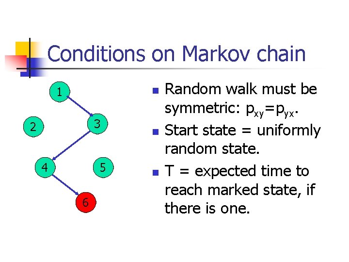
Conditions on Markov chain 1 n 3 2 4 5 6 n n Random walk must be symmetric: pxy=pyx. Start state = uniformly random state. T = expected time to reach marked state, if there is one.

Main result [Szegedy, 04] Theorem Assume that: 1. There are no marked states, or 2. A marked state is reached in expected time at most T. A quantum algorithm can distinguish the two cases in time O( T). Quadratic speedup for a variety of problems.

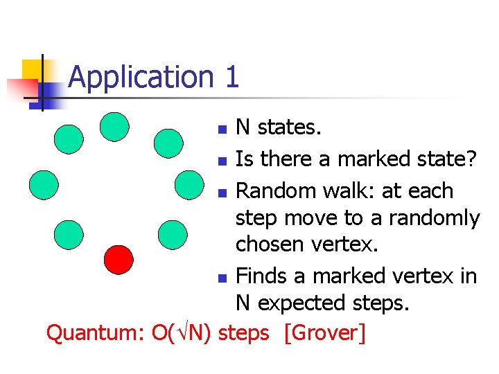
Application 1 N states. n Is there a marked state? n Random walk: at each step move to a randomly chosen vertex. n Finds a marked vertex in N expected steps. Quantum: O( N) steps [Grover] n

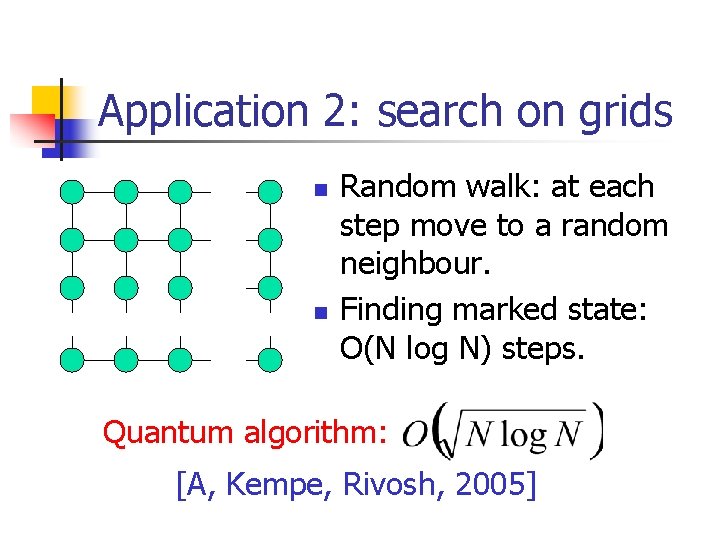
Application 2: search on grids n n Random walk: at each step move to a random neighbour. Finding marked state: O(N log N) steps. Quantum algorithm: [A, Kempe, Rivosh, 2005]

Application 3: element distinctness 7 9 2. . . 1 x 2 x 3 x. N n n Numbers x 1, x 2, . . . , x. N. Determine if two of them are equal. Well studied problem in classical CS. Classically: N steps.

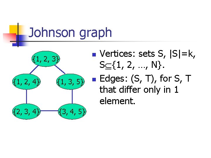
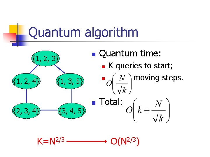
Johnson graph {1, 2, 3} {1, 2, 4} {1, 3, 5} {2, 3, 4} {3, 4, 5} n n Vertices: sets S, |S|=k, S {1, 2, …, N}. Edges: (S, T), for S, T that differ only in 1 element.

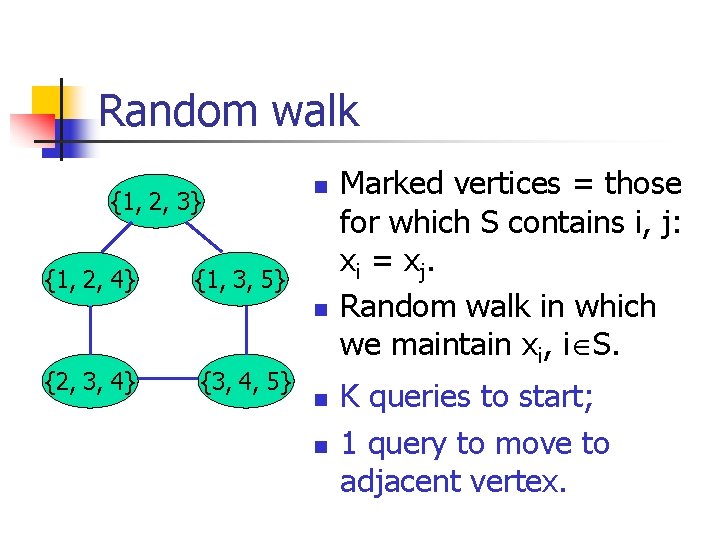
Random walk {1, 2, 3} {1, 2, 4} n {1, 3, 5} n {2, 3, 4} {3, 4, 5} n n Marked vertices = those for which S contains i, j: xi = xj. Random walk in which we maintain xi, i S. K queries to start; 1 query to move to adjacent vertex.

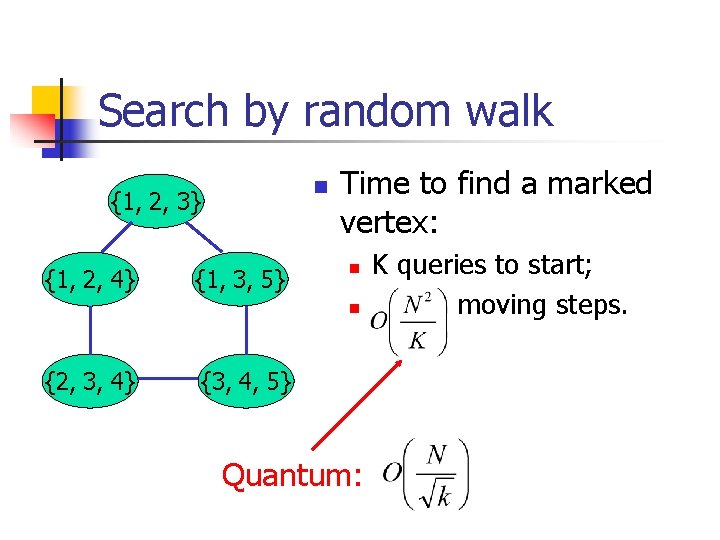
Search by random walk n {1, 2, 3} {1, 2, 4} {1, 3, 5} Time to find a marked vertex: n n {2, 3, 4} {3, 4, 5} Quantum: K queries to start; moving steps.

Quantum algorithm {1, 2, 3} n Quantum time: n {1, 2, 4} n {1, 3, 5} n {2, 3, 4} {3, 4, 5} K=N 2/3 K queries to start; moving steps. Total: O(N 2/3)

Triangle finding [Magniez, Santha, Szegedy, 03] n n n Graph G with n vertices. n 2 variables xij; xij=1 if there is an edge (i, j). Does G contain a triangle? Classically: O(n 2). Quantum: O(n 1. 3).

Matrix multiplication [Buhrman, Špalek, 05] n A, B, C – n*n matrices. Finding C=AB: O(n 2. 37…) steps; n Given A, B and C, we can test AB=C in: n n n O(n 2) steps by a probabilistic algorithm; O(n 5/3) steps by a quantum algorithm.

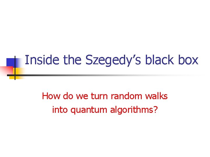
Inside the Szegedy’s black box How do we turn random walks into quantum algorithms?

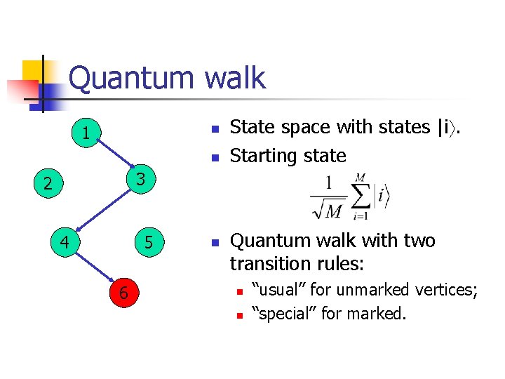
Quantum walk 1 n n State space with states |i. Starting state 3 2 4 5 6 n Quantum walk with two transition rules: n n “usual” for unmarked vertices; “special” for marked.

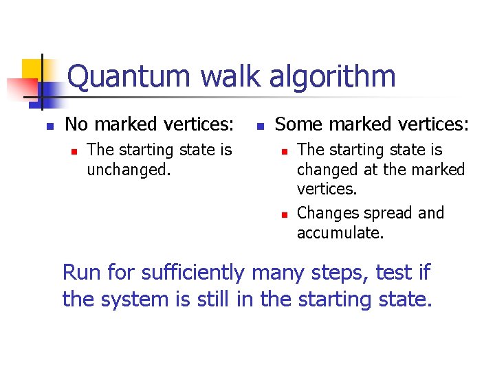
Quantum walk algorithm n No marked vertices: n The starting state is unchanged. n Some marked vertices: n n The starting state is changed at the marked vertices. Changes spread and accumulate. Run for sufficiently many steps, test if the system is still in the starting state.

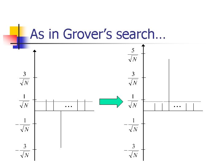
As in Grover’s search… … …

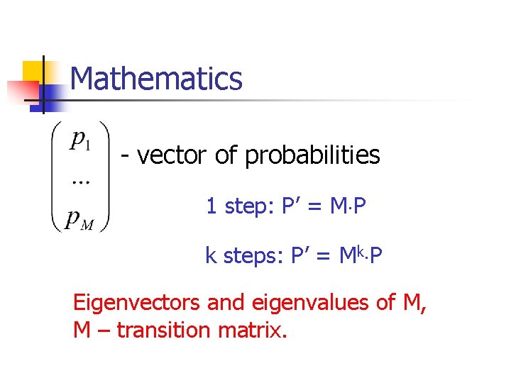
Mathematics - vector of probabilities 1 step: P’ = M P k steps: P’ = Mk P Eigenvectors and eigenvalues of M, M – transition matrix.

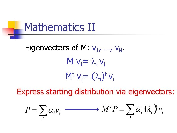
Mathematics II Eigenvectors of M: v 1, …, v. N. M v i = i vi Mt vi= ( i)t vi Express starting distribution via eigenvectors:

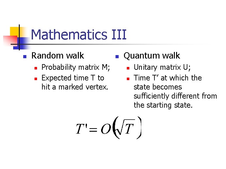
Mathematics III n Random walk n n Probability matrix M; Expected time T to hit a marked vertex. n Quantum walk n n Unitary matrix U; Time T’ at which the state becomes sufficiently different from the starting state.

Other applications of quantum walks

“Glued trees” [Childs et al. , 02] n n Two full binary trees of depth d; Randomly connect leaves of the two graphs.

“Glued trees” [Childs et al. , 02] n n Start position: the left root. Task: find the other root. Vertices and edges not labeled. 2 d+2 -2 vertices. Any classical algorithm takes (cd) steps.

“Glued trees” [Childs et al. , 02] n n Perform a quantum walk, starting from the left root. After O(d 2) steps, a quantum walk is at the right root. Exponential speedup: O(d 2) vs (cd).

[A, Childs, et al. , 07] n n AND n OR x 1 OR x 2 x 3 x 4 AND-OR formula of size M. Variables accessed by queries: ask i, get xi. Theorem Any formula can be evaluated with O(M 1/2+o(1)) queries. Speedup for anything that can be expressed as a formula

Conclusion n Quantum walks can be used to design quantum algorithms for many problems. Quantum walk search: create a classical random walk, quantize it with a speedup. “Quantum black box” within a classical algorithm.

Building a quantum computer n n n Classical computer operates on bits (0 or 1). Quantum bit: a system with basis states |0 , |1 , general state 0|0 + 1|1. Need physical systems that act like quantum bits… 10 s of candidates…

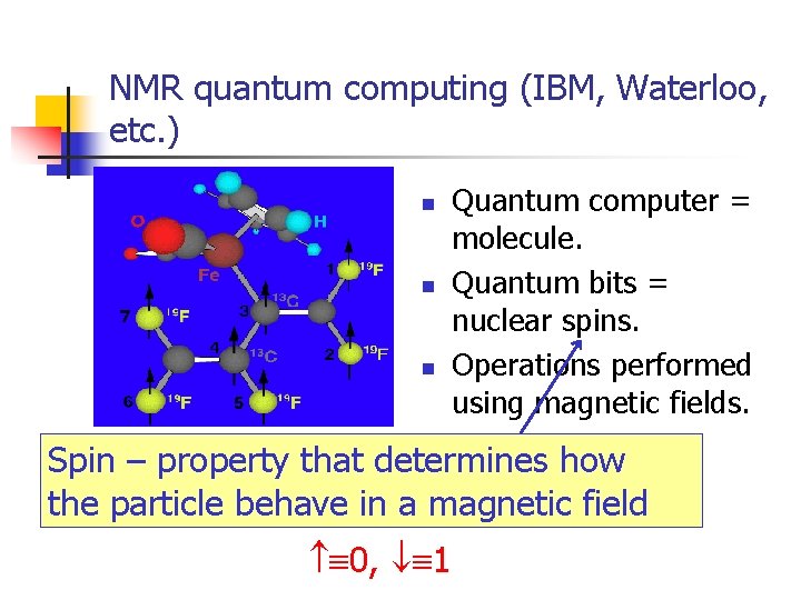
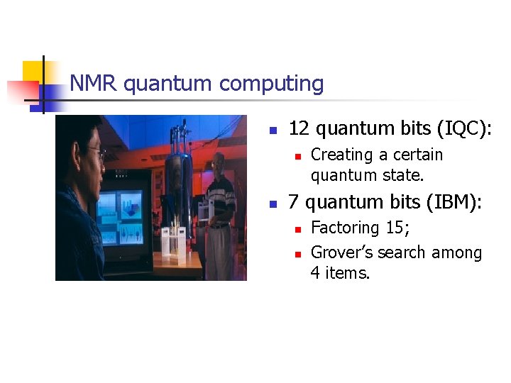
NMR quantum computing (IBM, Waterloo, etc. ) n n n Quantum computer = molecule. Quantum bits = nuclear spins. Operations performed using magnetic fields. Spin – property that determines how the particle behave in a magnetic field 0, 1

NMR quantum computing n 12 quantum bits (IQC): n n Creating a certain quantum state. 7 quantum bits (IBM): n n Factoring 15; Grover’s search among 4 items.

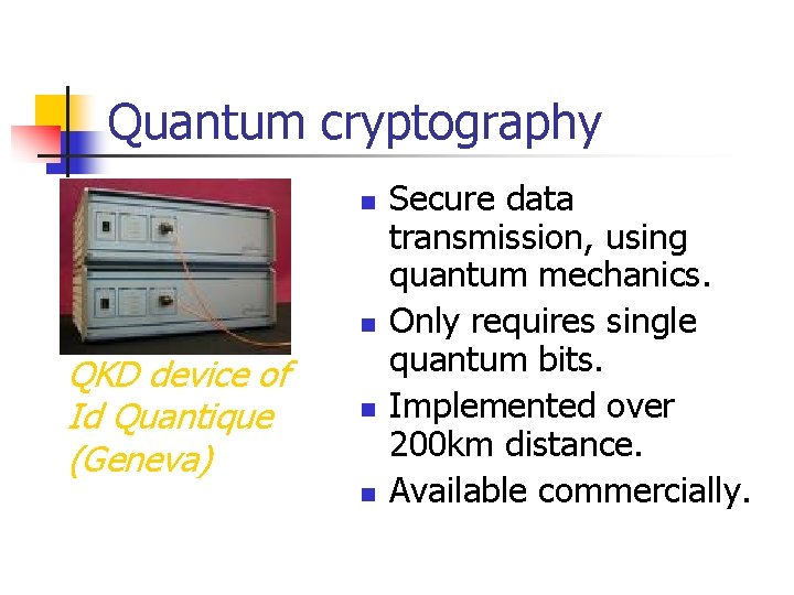
Quantum cryptography n n QKD device of Id Quantique (Geneva) n n Secure data transmission, using quantum mechanics. Only requires single quantum bits. Implemented over 200 km distance. Available commercially.