Quantum Mechanics 1 Birthday of Quantum Physics on

Quantum Mechanics 1

Birthday of Quantum Physics on 14 th December, 1900 On this date German physicist Max Planck first presented his new quantum concepts. Planck introduces a new fundamental constant Max Karl Ernst Ludwig Planck 1858 -1947 h to explain black-body radiation

Classical concept Two distinct categories : 1. Material body (particle) Newton’s laws of motion Position and velocity (momentum) are precisely measurable Spread over the space, amplitude gives 2. Electromagnetic field (wave) energy/intensity, frequency is nothing Maxwell’s equation but time periodicity of oscillator Additionally Laws of thermodynamics E = k. T Fundamental constants : 1. velocity of light c 2. Avogadro Number N 3. Boltzman constant k 4. Unit of charge e E = mc 2 Velocity << c : non-relativistic Velocity comparable to c : relativistic

Classical concepts never allow to think that 1. Wave may also behave like particle. (Planck’s hypothesis) 2. Particle may behave like wave. (de Broglie hypothesis) 3. Position and momentum of a particle cannot be measured accurately simultaneously. (Heisenberg uncertainty principle) 4. Energy of wave is related with frequency and quantised. n These new concepts are basically quantum concepts

BLACKBODY RADIATION The mother of Quantum Physics An ideal black body is an empty cavity whose walls are maintained at a given temperature T (at thermodynamic equilibrium)

BLACKBODY RADIATION The mother of Quantum Physics According to classical electrodynamics such a cavity has infinite number of normal modes. There is no upper limit to the frequency of these normal modes

Blackbody Radiation Classical thermodynamics predicts that at an equilibrium temperature T, the average amount of energy in a given normal mode is fixed = k. T Energy density in the window υ and υ +d υ ρ(υ) 3 J/m -Hz k=: Boltzmann’s const. = 1. 38 x 10 -23 T=1800 K T=1400 K T=1000 K frequency υ J/K

As there is no upper limit to the frequency of these normal modes, there would be infinite number of normal modes, and thus infinite amount of energy residing in the EM radiation within the cavity at a finite temperature. Ultraviolet catastrophe

Classical theory of Rayleigh-Jeans law The amount of energy per unit volume per unit frequency interval (Spectral density) should keep on increasing with frequency as 2. (Obeyed well at low frequencies) T=1800 K ρ(υ) T=1800 K T=1400 K T=1000 K frequency υ

ρ(υ) T=1800 K 2 υ dependence frequency υ

Rayleigh-Jeans law ρ(υ) Planck’s law frequency υ

EM radiation in black body is quantum field. The average energy in a normal mode is of the order of k. T. The probability of emission of high energy photons with high frequency gets smaller for a given temperature when h >> k. T. There is not enough energy available for emitting these photons.

Planck’s Radiation Law The density of radiant energy in the cavity per unit wavelength interval, at the wavelength , and at the temperature T

Planck’s Formula Rayleigh-Jeans law

Planck’s postulate Any physical entity with one degree of freedom and whose ``co-ordinate” is oscillating sinusoidally with frequency can possess only total energies E as integral multiple of h. h = Planck’s constant 4 2 Classical E=0

Waves behaving as particles Experiments 1. Photoelectric effect (1902) 2. Compton effect (1922) 3. Pair Production

particle wave duality de Broglie postulate

Particles behaving as waves Experiments Electron diffraction Davisson –Germer (USA) and Thompson (UK) (1927) Electron microscope

Photoelectric effect

Photoelectric effect

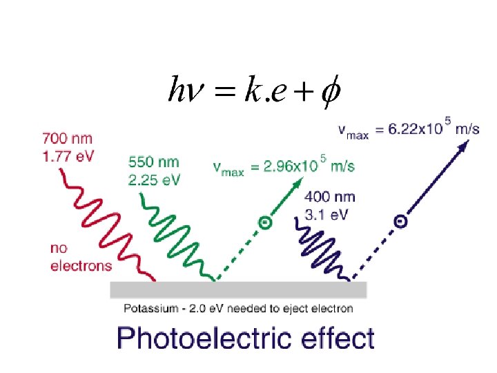
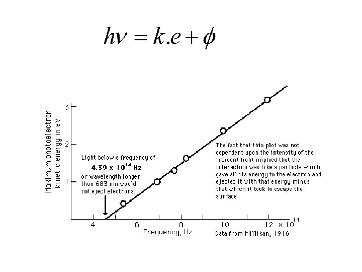
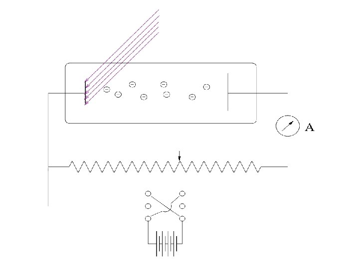
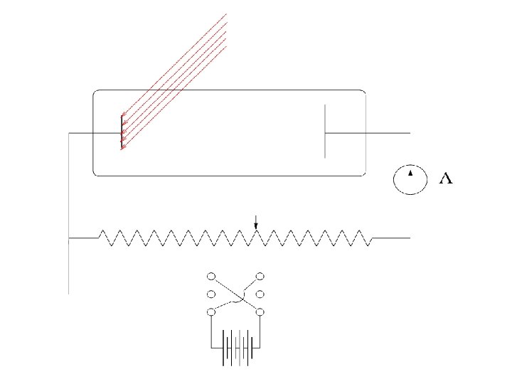
Lenard 1902: Studied energy of the photoelectrons with intensity of light. He could increase the intensity thousand fold. 1. Noticed a well defined minimum voltage Vstop to stop the current in the circuit. Vstop was independent of the intensity of light.

Current vs Voltage Different intensities: Ib > Ia Cut-off voltage

2. Increasing the intensity of light would increase the current 3. He performed the experiment with various coloured lights and found the maximum energy of the electrons did depend on the frequency of light. Qualitatively he obtained more the frequency more the energy.

Objections with wave theory 1. Kinetic energy (K) of the photo-electron should increase with intensity of the beam. But Kmax was found to be independent of the intensity of the falling light.

2. Effect should occur for any frequency of light provided only that light is intense enough to eject the electron. But a cut-off frequency was observed below which photoelectrons were not ejected (no matter how intense was beam).

3. Energy in the classical theory is uniformly distributed over the wave front. If light is feeble, there should be a time lag between the light striking the plate and ejection of photoelectrons. Ejection is instant, t < 10 -9 sec

Einstein equation

Light is wave : Interference, Diffraction, polarisation Light is a stream of photons/wave packets (particles) So wave behaves like particle

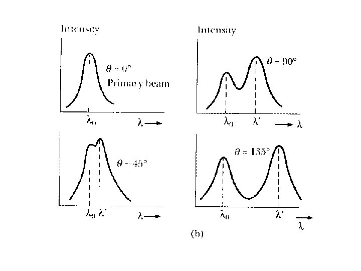
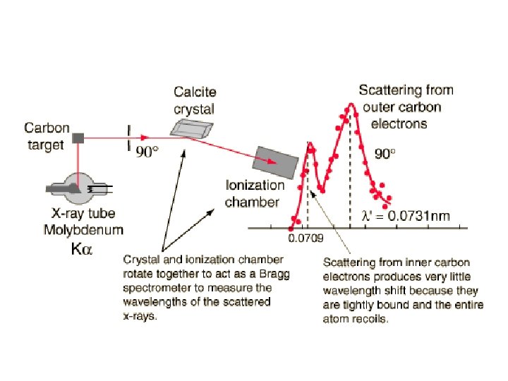
Compton effect Collision between photon and electron

Compton Effect in 1920 Arthur Holly Compton (1892 -1962)

Partial transfer of photon energy

m = m(v) is the relativistic mass

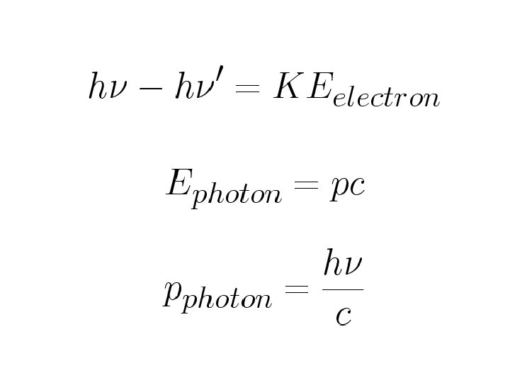
Conservation of momentum along initial photon direction Conservation of momentum along perpendicular to initial photon direction Square and add the above two expressions

Energy conservation

Compton shift ~ Compton wavelength = 2. 4 pm

Compton Experiment

Pair production (Energy into matter) Nucleus The rest mass of e- or e+ is 0. 51 Me. V. Hence pair production requires a photon energy of at least 1. 02 Me. V. Corresponding max. photon wavelength is 1. 2 pm (Gamma rays) The linear momentum is conserved with the help of the nucleus In empty space momentum and energy cannot be simultaneously conserved θ θ

Pair annihilation is inverse of Pair production Compton scattering

Confirmation of discrete energy levels in atom Franck and Hertz experiment (1914) (James Franck and Gustav Hertz)

Vo

Peaks at 4. 9 V and its multiples 300 200 I in m. A 100 5 10 15 Accelerating Voltage in Volts

Continuum E=0 2 nd excited state 1 st excited state 6. 7 e. V Ground state 4. 9 e. V E= -10. 4 e. V

Particles behaving as waves Experiments Electron diffraction Davisson –Germer (USA) and Thompson (UK) (1927)

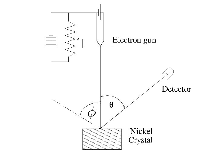
Diffraction?

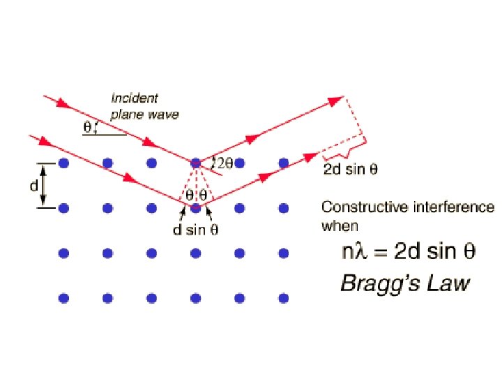
Apply Bragg’s law From X-ray diffraction

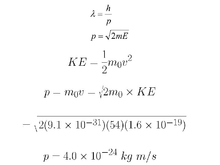
de Broglie wavelength of electron KE=54 e. V is non relativistic

Bohr’s Complementarity Principle “In a situation where the wave aspect of a system is revealed, its particle aspect is concealed; and, in a situation where the particle aspect is revealed, its wave aspect is concealed. Revealing both simultaneously is impossible; the wave and particle aspects are complementary. ”

W. Heisenberg Uncertainty relations & Matrix mechanics (1932) E. Schrödinger Wave mechanics (1933)

P. A. M. Dirac Relativistic theory of electron (1933) W. Pauli Exclusion principle (1945)

Heisenberg’s Uncertainty Relations Minimum Uncertainty (Gaussian wave packets) Single-slit diffraction: x in slit-width, changes px

This principle is of great importance in understanding many phenomena Electrons confined in atoms

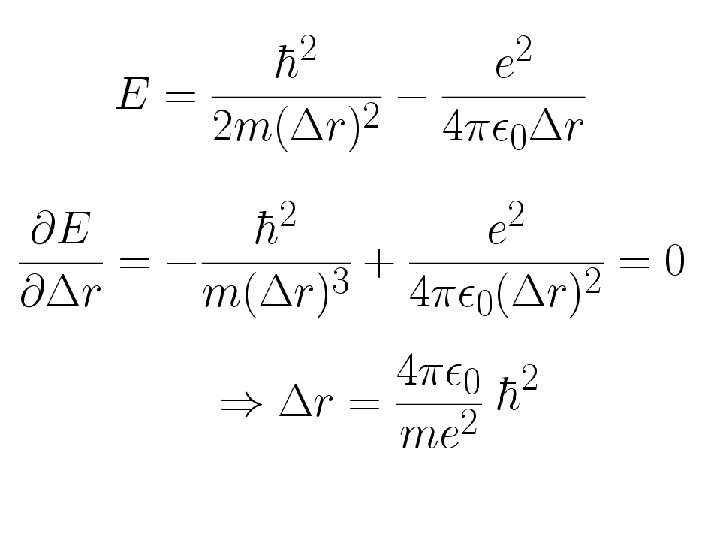
J e. V Hydrogen atom ionisation potential : 13. 6 e. V Calculate the energy of e- if it were to be in the nucleus: x ~ 10 -15 m

This principle is of great importance in understanding many phenomena particles confined in nucleus Size of the nucleus

This principle is of great importance in understanding many phenomena Harmonic oscillator: Ground state

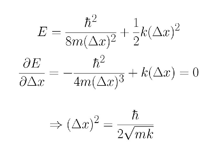
Zero point energy

This principle is of great importance in understanding many phenomena Hydrogen atom: Ground state

Bohr radius Minimum energy

Classical physics is deterministic Quantum physics/mechanics is probabilistic

Consider single-slit diffraction (photon or electron): - With a single particle the diffraction pattern is absent. - When the experiment is repeated with large number of particles the diffraction pattern is observed. Q: So, where does the particle go after passing through the slit? Ans: It has a large probability to go where there is a diffraction maxima.

For a classical system made up of particles: a) Position and momentum (or equivalently velocity) are specific at any particular time. b) If position and momentum is known at an initial time, then if you know all the forces acting on that particle you can write down equations which tell you exactly what its position and momentum will be at any future time. c) Note that instead of specifying the forces you can specify the potential energy function, which is equivalent: force is the gradient of potential.

In quantum mechanics the situation is a little more complicated The systems that you study are still made of particles, and the basic procedure is in some ways similar: a)You measure the state of a particle at some initial time, you specify the forces acting on that particle (or equivalently, the potential energy function describing those forces), and quantum mechanics gives you a set of equations for predicting the results of measurements taken at any later time. b) There are two key differences between these two theories. à the state of a particle in quantum mechanics is not just given by its position and momentum but by something called a "wavefunction. " à knowing the state of a particle (i. e. , its wavefunction) does not enable you to predict the results of measurements with certainty, but rather gives you a set of probabilities for the possible outcomes of any measurement. The wave-function is a complex function which is defined everywhere in space. No matter what state your particle is in, its wave-function has some complex value at every point in the universe.

Basic postulates of Quantum mechanics Probabilities in QM are determined from wave functions (not observable) Complex Wavefunction 2 Observable Well behaved must be continuous and single-valued everywhere / x must be continuous and single-valued everywhere must go to zero as x ±

Probability of finding the particle between

x

2 1 2 =P(1, 2) x

Superposition If 1 and 2 are two wavefunctions that satisfy the equation, then 1+ 2 is also a solution, where a and b are constants.

A typical quantum mechanics problem would thus run as follows: i) You start with a particle in an unknown state subject to a known set of forces, such as an electron in an electromagnetic field. ii) You perform a measurement on that particle that tells you its state, i. e. , its wavefunction. iii) You let it evolve for a certain amount of time and then take another measurement. iv) Quantum mechanics can tell you what result to expect from this second measurement.

Position probabilities with a discrete wavefunction • How do you use to predict the results of a measurement of the particle's position? • A simple case Suppose a particle can exist in only three points: x=1, x=2, and x=3. Our particle must be on exactly one of those points. It cannot be anywhere else, including in between them. So is just three complex numbers, which might look something like this. x = 1: = 1 + i x = 2: = 2 - 2 i x = 3: = 2 + 2 i

• | |2 gives the probability of finding the particle at a particular position. • The probability of finding our particle at position x=1 is |1+i|2 which is 2. The probability of x=2 is 8. So, for any given measurement, we are four times as likely to find the particle at position 2 as at position 1. • Now, if we sum up the probabilities of all three locations, we get the odds that the particle will be in any one of those three states. Since we've already said that the particle must be at one of those states, we should get a probability of 1.

• But at the moment, we find a total probability of 18! • This wavefunction is unnormalized: • It can tell us the relative probabilities of two positions, but not the absolute probabilities of any of them. • To normalize it, we multiply all the values by a constant, to make the total probability equal to 1. • In this case, we have to multiply every value of | |2 by 1/18, which means we multiply every value of by the square root of 1/18. This will keep all the relative probabilities the same, but ensure that the total probability of finding the particle somewhere is 1.

• So now, at our three places, we have the following. x=1, probability=2/18 x=2, probability=8/18 x=3, probability=8/18 • That is a properly normalized description of the particle's position. You can't say for sure what any given measurement will find, but you know exactly what the odds are.

Therefore the wave-functions at the three places can be written as: probability=2/18 probability=8/18

• “Expectation value" of position Expectation value < x > of the position of a particle described by wave function (x, t), is the value of x we would obtain if we measured the position of a large number of particles described by the same wavefunction at some instant t and then averaged the results. It is not the most probable value of a measurement.

For a large number of identical particles, distributed along x-axis so that there are N 1 particles at x 1, N 2 at x 2 etc…: The average position of the identical particles: If we deal with single particle, we must replace Ni of particles at xi by the probability Pi, that the particle be found in interval dx at xi. where i is the particle wave-function at x=xi.

Expectation value of the position of a single particle is: If is normalised wave function, Evaluate the expectation values: <E> and <p> ?

Problem: A particle limited to the x-axis has the wave function = ax between x = 0 and x = 1; = 0 elsewhere. (a) Find the probability that the particle can be found between x = 0. 45 and x = 0. 55. (b) Find the expectation value <x> of the particle’s position. Solution: (a) The probability is: (b) The expectation value is:

Consider a free particle wave function: Knowing that E = ħ and p = ħk

Successive differentiation will give and Now for a free non-relativistic particle E = p 2/2 m

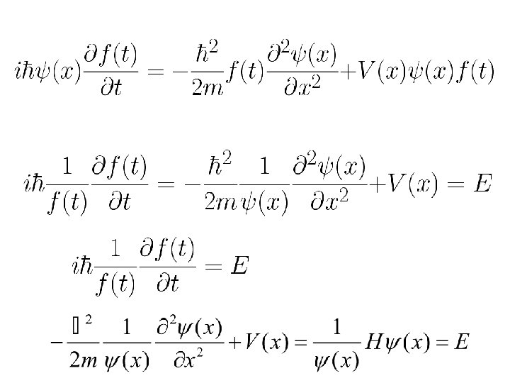
Therefore, we have This is the one-dimensional time dependent Schrödinger equation for a free particle. We also get that E and p can be represented by:

Till now we have assumed the particle to be free. If we now assume the particle to be in a field characterized by the potential energy function V(x, t) then according to classical mechanics, the total energy would be given by: E= p 2/2 m + V(x, t) Since the potential energy function does not depend on p and E, we have from preceeding two important equations that the wave-function should satisfy Where H= p 2/2 m + V and is known as the Hamiltonian.

Shrödinger Equation For conservative systems having time-independent potential energy V(x): Separation of variables

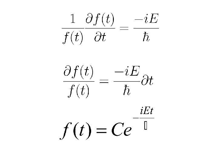
Note that t in the above equation is only a phase factor. It does not effect the probability distribution or expectation value. As t does not appear in the measurable quantities the eigenstates of the time-dependent Schrödinger equation of a conservative system are known as the stationary states.

Time independent Schrödinger eqn.

One dimensional Potential well V 0 Infinite L -V 0 V(x)= 0 for 0<x<L =∞ for x<0 and for x>L

The one dimensional Schrödinger equation becomes The general solution of this equation is: ψ=A sin kx + B coskx The boundary condition is ψ(x=0) = ψ(x=L) = 0 Using this condition, you will get that B=0 and A is either 0, or k. L= nπ.

The condition that A=0 leads to the trivial solution of ψ vanishing everywhere, the same is the case for n=0. Thus the allowed energy levels are given by

For the nth energy level the wavefunction is given by: Before finding the probability amplitude, we have to normalize the wavefunction to unity The corresponding eigen-functions are: Eigenfunctions are the wavefunctions associated with the eigenvalues:

The complete time-dependent wave function is:

L -V 0

Finite depth well V 0 Finite L -V 0

One dimensional Potential step E > V 0 E < V 0 x

One dimensional Potential barrier Quantum mechanical tunneling E < V 0 x More the barrier height less the transmission probability More the barrier width less the transmission probability

Applications in atom trapping experiments

THE END