Quantum Distribution Functions for Bosons Fermions otherwise Objects

Quantum Distribution Functions for Bosons, Fermions, & otherwise Objects

How to do the Lagrange Multiplier technique Maximize a function subject to certain constraints on the dependent variables • function f(x 1, x 2, …) • Constraint g(x 1, x 2, …)=c • Form new function F = f + l (g-c) • Maximize/Minimize it wrt x 1, x 2, … • Choose something for l based upon other information http: //www. slimy. com/~steuard/teaching/tutorials/Lagrange. html http: //www. cs. berkeley. edu/~klein/papers/lagrange-multipliers. pdf

Example Minimize f = xy subject to constraint x 2+y 2=1 F = xy + l (x 2+y 2 -1) d. F/dx = y + 2 lx (y+2 lx) + (x+2 ly) = 0 (1+2 l)y + (1+2 l)x = 0 d. F/dy = x + 2 ly y = -x x 2+y 2=1 x 2+x 2=1 2 x 2 = 1 x=± 0. 707

OUTLINE • • • Harris 8. 1 – Quick Basic Probability Ideas Harris 8. 4 -8. 5 – Derivation of Boltzmann Distribution Fn – How to Use it – How to Normalize it Harris 8. 2 -8. 3 Macroscopic Descriptions – Entropy and Temperature – Density of States Harris 8. 6 – Comparison of Ytot* Ytot for Bosons & Fermions – Detailed Balance • w/o special requirements • bosons • fermions – Distribution Fns • Interpreatations of the ea factors Harris 8. 7 -8. 10 – 8. 7 Density of States, Conduction Electrons, Bose-Einstein Condensation – 8. 8 Photon Gasses – 8. Laser Systems – 8. 10 Specific Heats

Harris 8. 1 Thermodynamic Systems

Microinfo vs Macroinfo { ri, pi, Li, Si, Ei, …} i = 1, …, hugen number Etot, P, V, T, N, …

Microstates vs Macrostate Very few microstates are similar to this Most Probable arrangement Many microstates are similar to this # collection of most probable microstates should be described with macro-parameters P, V, N, T, Etot, … S = k. B ln W

• Systems where microscopic approach is limited – Solids – 3 -body problems in ‘planetary’ motion – Hartree-Fock Procedure • Multielectron atomic structure • Nuclear Structure • e Each system has it’s own macroscopic parameters, but the set always includes Ntot , Etot, Ave Kinetic Energy (~T).

What is most likely arrangement of 4 balls in 2 bins?

BACKGROUND PROBABILITY IDEAS

Given N=5 objects and p=1 bin; How many ways can one put n=2 objects in the bin ? (in a definite order)

Given N=5 objects and p=1 bin; How many ways can one put n=2 objects in the bin ? (without regard to order) Note that after filling this box, there are (N-n) objects unused.

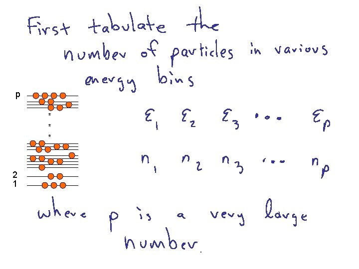
Given N total objects and p total bins; How many ways can one put n 1 objects in bin #1 n 2 objects in bin #2 n 3 objects in bin #3 *** (without regard to order) * * *

* * * n 1 n 2 n 3

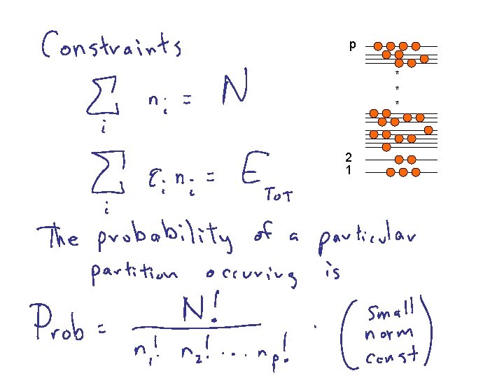
Probability of finding a particular arrangement:

Probability Summary N total objects p total states np n 5 n 4 n 3 n 2 n 1 * * *

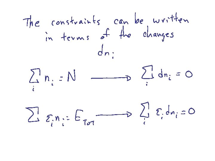
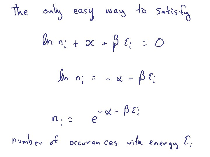
Harris 8. 4 BOLTZMANN DISTRIBUTION Probability of finding a particular energy e subject to the constraint that there are N total particles and Etot energy

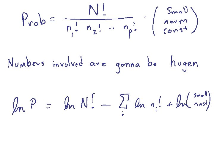
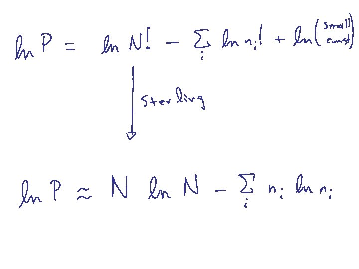
Sterling’s Formula The second term is largest by at least a parsec

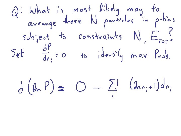
note: reset 1 + a a

To discover the expression for the normalization constant (assume smooth spectrum) OK, so what is b = ?

Temperature is defined in terms of the average kinetic energy

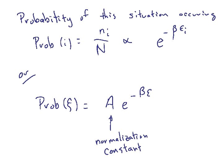
Boltzmann Distribution Probability of finding a particular energy e subject to the constraints that there are N total particles and fixed Etot ea = 1/k. T

How to normalize the Boltzmann Distribution and Density of States

We normalized the Boltzmann distribution assuming all energies could occur Prob = e-a e-E/k. T = A e-E/k. T

Many, many possible states, closely spaced in energy Just did this

Finite number of states, but no restriction on filling * * *

Density of States conduction band valence band core electrons

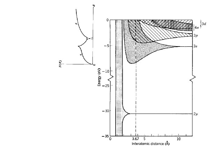
Density of states D(E) = # states per Energy interval Isolated Na Na as solid Density of States

Calculating Averages if were motivated enough to normalize ND beforehand if decided to do it later

Many, many closely-spaced states, but with restriction on filling Just did this

Finite number of states, but with restriction on filling * * * w 5 w 4 w 3 w 2 w 1 D(e) is funky notation, so use wi

Harris 8. 2 -8. 3 Macroscopic Descriptions Entropy & Flow of Time James Sethna @ Cornell: Chapter 5 http: //pages. physics. cornell. edu/sethna/Stat. Mech/Entropy. Order. Parameters. Complexity. pdf http: //www. tim-thompson. com/entropy 1. html http: //en. wikipedia. org/wiki/Entropy_%28 statistical_thermodynamics%29 http: //en. wikipedia. org/wiki/Entropy http: //en. wikipedia. org/wiki/Ludwig_Boltzmann http: //en. wikipedia. org/wiki/Satyendra_Nath_Bose http: //en. wikipedia. org/wiki/Fermi_distribution

Types of Entropy is what an equation defines it to be. Wiki: Carnot • Thermodynamic Entropy H (8 -3) • Statistical Mechanics Entropy Wiki: boltz H (8 -2) • Information Entropy http: //en. wikipedia. org/wiki/Entropy_%28 statistical_thermodynamics%29

Shannon quote (1949): The theory was in excellent shape, except that he needed a good name for “missing information”. “Why don’t you call it entropy”, von Neumann suggested. “In the first place, a mathematical development very much like yours already exists in Boltzmann’s statistical mechanics, and in the second place, no one understands entropy very well, so in any discussion you will be in a position of advantage. Wiki: History_of_Entropy

Stat Mech Example S = k. B ln(#microstates) S = k. B ln(1) S=0 S = k. B ln(4) S = 1. 38 k. B S = k. B ln(6) S = 1. 79 k. B

Stat Mech Example p 1 = 0. 25 p 3 = 0. 25 p 2 = 0. 25 p 4 = 0. 25 pi = 0. 167 pi = 1 S=- k. B 1 ln(1) = 0 S = 1. 38 k. B S = 1. 79 k. B

Flow of Time Changes between microstates are generally easily reversible. It is not necessarily likely that changes between macrostates can be reversed.

Harris 8. 6 Back to Probability Distributions

COMPARING PROBABILITIES Y*Y for Indistinguishable Boson/Fermion Particles to those without worrying about B/F requirements

Distinguishable Particle Probabilities One particle in a state b Ytot = Yb(1) Prob = Ytot* Ytot = Yb(1) * Yb(1) = 1 Two particles in a state b Ytot = Yb(1) Yb(2) Prob = Yb(1)* Yb(1) Yb(2)* Yb(2) = 1 Three particles in a state b Ytot = Yb(1) Yb(2) Yb(3) Prob = Yb(1)* Yb(1) Yb(2)* Yb(2) Yb(3)* Yb(3) = 1 So what ? Nothing special happens here…. .

Indistinguishable Boson Probabilities One particle in a state b Ytot = Yb(1) Prob = Ytot* Ytot = Yb(1) * Yb(1) = 1 Two particles in a state b Ytot = [Yb(1) Yb(2) + Yb(2) Yb(1)] = 2 Prob = |2 Yb(1) Yb(2) |2 = 2! Three particles in a state b Ytot = [ Yb(1) Yb(2) Yb(3) + … ] Prob = | 6 Yb(1) Yb(2) Yb(3) |2 = 6 = 3! If there already n bosons in a state, the probability of one more joining them is enhanced by (1+n) than what the prob would be w/o indistinguishability requirements

Indistinguishable Fermion Probabilities One particle in a state b Ytot = Yb(1) Prob = Ytot* Ytot = Yb(1) * Yb(1) = 1 Two particles in a state b Ytot = [Yb(1) Yb(2) - Yb(2) Yb(1)] = 0 Prob = 0 If there already n fermions in a state, the probability of one more joining them is enhanced by (1 -n) than what the prob would be w/o indistinguishability requirements

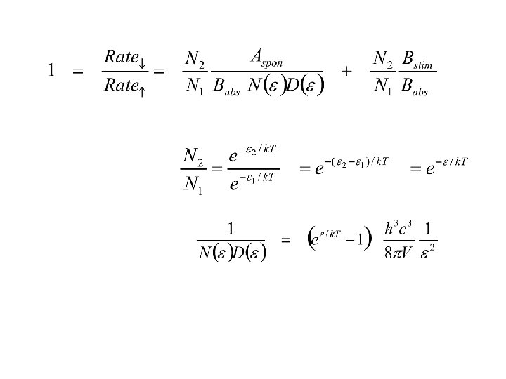
Principle of Detailed Balance For two states of a system with fixed total energy, n 2 e 2 n 1 e 1 Where the particles can jump between states by some unknown mechanism, Rate of upward going transitions = Rate of downward going transitions n 1 Rate 1 2 = n 2 Rate 2 1 transitions/sec per particle

Detailed Balance distinguishable particles (but with no other special requirements) Since by the Boltzmann distribution n ~ e-e/k. T Gives us the ratio of the two transition rates

Detailed Balance indistinguishable bosons

L & R sides are unrelated except for Temp

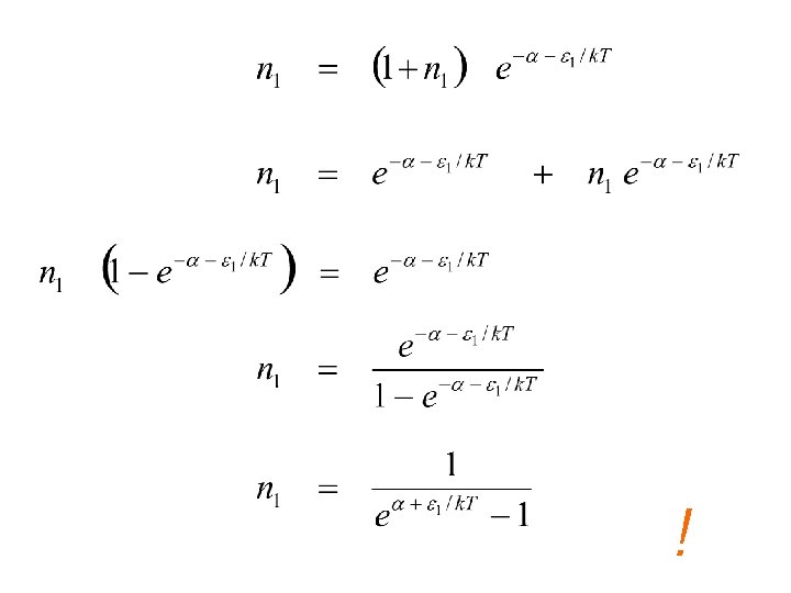
Bose distribution function Probable # bosons of an energy e in a system of fixed total energy at a temperature T

Detailed Balance indistinguishable fermions ( short derivation )

Fermi distribution function Probable # fermions of an energy e in a system of fixed total energy at a temperature T

SUMMARY of Distribution Functions and what is this a thing?

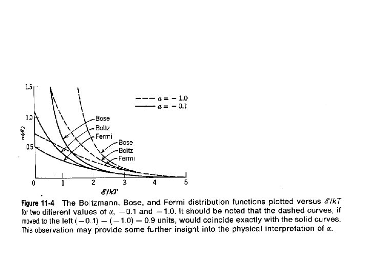
Collected Distribution Functions Boltzmann Bose Fermi

Normalization Interpretation Boltz ea = k. T a = a real mess Bose * a = a real mess Fermi * This interpretation may not be so useful for Bose & Fermi distributions * For N tot free particles strictly confined to a 3 -D region of space of volume V.

Chemical Potential Interpretation m = - a k. T Boltz ea = e-m/k. T Bose ea = e-m/k. T Fermi ea = e-m/k. T A uniform description for all three distributions. Used for Bose distribution.

• Problem: chemical potential is not an easily measured or well understood quantity most people) (by – Defn: How the total energy of a system changes as one changes the count of objects – How does the total NRG change if we replace a 10 e. V photon with two 5 e. V photons? Ans: it doesn’t, m=0. this system is called a photon/phonon gas – How does the total NRG change if we replace a KE 10 e. V proton with two 5 e. V protons? Ans: some – How does the total NRG change if we replace a KE 10 e. V H-atom with two 5 e. V H-atoms? Ans: a v. s. amount

50% Probability Interpretation At what energy is the probability 50% of it’s maximum value? (called the Fermi energy ef ) Boltz Not used Bose Not used when e = ef Fermi Used for Fermi distribution.

Summary of Common Usage Probability Boltz ea = k. T Chemical Potl Bose m Fermi Energy Fermi ef

Boltzmann normalization interpretation ea = 1/k. T

Bose for phonon gas chemical interpretation m=0

Fermi ½ value interpretation a = -ef / k. T

EXAMPLES OF QUANTUM GASES & FLUIDS Harris 8. 7 -8. 10 • • Density of States in a 3 D bound system (massive objects) Electron Gas: Conduction Electrons Photon Gas: Blackbody Spectrum Gas Laws: ‘PV=n. RT’ Bose Gases: 4 He Bose-Einstein Condensates Specific Heat of Solids Laser Systems

Density of States in 3 D confined system Harris 8. 7

In a 3 D slab of metal, e’s are free to move but must remain on the inside Solutions are of the form: With nrg’s:

At T = 0, all states are filled up to the Fermi nrg A useful way to keep track of the states that are filled is:

total number of states up to an energy efermi: 2 s+1 2 spin states Harris (8 -43) # states/volume ~ # free e’s / volume

Sample Numerical Values for Copper slab = 8. 96 gm/cm 3 1/63. 6 amu 6 e 23 = 8. 5 e 22 #/cm 3 = 8. 5 e 28 #/m 3 efermi = 7 e. V nmax = 4. 3 e 7 efermi = 7 e. V

Density of States How many combinations of are there within an energy interval e to e + de ? Harris (8 -40)

Electron Gas Conduction Electrons Harris 8. 7

At T ≠ 0 the electrons will be spread out among the allowed states How many electrons are contained in a particular energy range? N(e) D(e)

this assumes there are no other issues

Distribution of States: Simple Free-Electron Model vs Reality

Photon Gas Harris 8. 8

Photon Gas -- Harris 8. 8 distrib fn Number of ways to have a particular energy

Photon Gas Bose m=0 1. Factor of 2 for polarization states

Photon Gas integrand is the ~ intensity at an energy e a. k. a. Planck’s Blackbody Spectrum

Photon Gas Stefan-Boltzmann Law Radiated Intensity = s T 4 W/m 2 s = 5. 67 E-8 Wien Displacement Law lmax. T = 2. 898 E-3 m*K

‘Ideal’ Gas Laws

GASES ‘PV=n. RT’ Boson / Fermion / don’t care distrib fn Number of ways to have a particular energy

don’t care Gases N(e) = Boltzmann distrib ½ k. T KE per degree of freedom

Boson Gases N(e) = Bose distrib Small 10 -5 at STP Derivation assumes gas lives in 3 D box, infinite square well Harris (8 -42)

Boltz Bose

Fermi Gases N(e) = Fermi distrib Derivation assumes gas lives in 3 D box, infinite square well Small 10 -5 at STP

Boltz Fermi

Can we find a gas that would exhibit Boson effects ? small mass m, low Temp, high density Ntot / V H 2 at condensation point 20 K e-a ~ 1/100 He at condensation point 4. 2 K e-a ~ 1 / 7

Liquid He Phonon gas – intra atomic interactions helium common 26 atm • Very low viscosity • Density = 0. 125 g/cc (1/4 of what expected) • nrg of thermal motion ~ nrg of inter-atomic effects 0. 5 me. V

Liquid He Not really a gas, but hey… below Tl helium common 26 atm • Heat is conducted through liquid w/o thermal resistance ( drops by 106 at Tl) • Viscosity of fluid drops suddenly ( drops by 106 at Tl) • Bulk ordered mass motion. Creep at ~ 30 cm/s

Below 4. 2 K, Heat is conducted without boiling.

Creep

• Liquid Helium Film Creep – http: //www. youtube. com/watch? v=fg 1 hu. Roa. Jd. U • Helium below l-point – http: //www. youtube. com/watch? v=TBi 908 sct_U – http: //www. youtube. com/watch? v=YKj. FPpu. K-Jo • s

wikipedia Helium I has a gas-like index of refraction of 1. 026 which makes its surface so hard to see that floats of Styrofoam are often used to show where the surface is. [5] This colorless liquid has a very low viscosity and a density 1/8 th that of water, which is only 1/4 th the value expected from classical physics. [5] Quantum mechanics is needed to explain this property and thus both types of liquid helium are called quantum fluids, meaning they display atomic properties on a macroscopic scale. This is probably due to its boiling point being so close to absolute zero, which prevents random molecular motion (heat) from masking the atomic properties. [5]

wikipedia Boiling of helium II is not possible due to its high thermal conductivity; heat input instead causes evaporation of the liquid directly to gas. Helium II is a superfluid, a quantum-mechanical state of matter with strange properties. For example, when it flows through even capillaries of 10 -7 to 10 -8 m width it has no measurable viscosity. However, when measurements were done between two moving discs, a viscosity comparable to that of gaseous helium was observed. Current theory explains this using the two-fluid model for Helium II. In this model, liquid helium below the lambda point is viewed as containing a proportion of helium atoms in a ground state, which are superfluid and flow with exactly zero viscosity, and a proportion of helium atoms in an excited state, which behave more like an ordinary fluid. [6] A short explanation for the phenomenon would be that in this state, the temperature of the Helium is so low that almost all Helium atoms are in the lowest (quantum mechanical) energy state. Since energy can only be lost in discrete steps, and atoms in the lowest state cannot lose any energy, gravity and friction have no effect on single atoms.

Bose Condensates -- kinda Harris 8. 7 http: //www. colorado. edu/physics/2000/bec Java Applet: Thermal Box Java Applet: Thermal Quantum Well Java Applet Evaporative Cooling Animated gif of Condensation Interference of Two BEC Manipulation of BEC by Optical Lattices Quantum Computing ‘Slow Light’ 17 m/s

Specific Heats of Solids Harris 8. 10

SPECIFIC HEAT of Solids at Normal Temps k. T of Tot E (=KE+U) per dof Specific Heat law of Dulong & Petit

Specific Heat of Solids at Lower Temps 1) Einstein treatment incorrect T dependence 2) Debye treatment • Fe Q = 465 K • Al Q = 395 K • Ag Q = 210 K

Classical: Dulong & Petit Einstein’s approach: fudge it with Planck’s bb distribution But it didn’t get the very low temp CV correct Peter Debye worked it out with the distribution functions

Specific Heat of Solids at Lower Temps Boltzmann -- atom sites are distinguishable number of states of energy e, properly normalized (Debye model)

Laser Systems Harris 8. 9 1. Two State System 2. Forcing a Population Inversion 3. Examples Desired outcome: Light Amplification by Stimulated Emission of Radiation

Two State Detailed Balance N 2 E 2 N 1 E 1

N 2 N 1 Incoming photon just as likely to knock one down as knock one up -- as long as system is in equilibrium. Light Amplification by Stimulated Emission of Radiation

Back up to: 1 Light Amplification by Stimulated Emission of Radiation

History of Light Amplification • • 1953 Townes, Gordon, Zeiger: microwave amp 1955 Basov, Prokhov: 3 state 1957 Townes, Schawlow: change to optical 1957 Gould: design sketches 1959 Gould: “laser” and practical apps 1960 Maiman first working laser 1960 -1987 Gould vs Townes court battles

Mechanisms for “pumping” a Population Inversion N 2 >> N 1 fast • • Xe Flash lamp Electrical discharge Collisional excitation: He. Ne Laser of another frequency Chemical Laser Excimer Laser Q-switching Solid State Semiconductor Metastable t=long xxxxxxx fast

Ruby Laser Theodore Maiman 1960 blue band • Cr in Al 2 O 3 • • Ruby ends flat to 1/3 l Ruby ends polished to form Fabry-Perot • • • Xe flash lamp Cr+++ absorbs ~550 nm Cr+++ metastable ~3 ms green band 3 ms http: //laserstars. org/history/ruby. html

He. Ne http: //www. recycledgoods. com/item/18303. aspx He. Ne game http: //phys. educ. ksu. edu/vqm/html/henelaser. html http: //www. shopeio. com/inventory/details. asp? id=953

He. Ne 1 s 2 s 1 S 3 S 0 20. 61 e. V 5 s 4 s 1 20. 66 e. V 20. 30 e. V 4 p 19. 78 e. V 18. 70 e. V 3 p 3 s 16. 70 e. V 1 s 1 s He Ne 1 s 22 s 22 p 6 http: //repairfaq. ece. drexel. edu/sam/MEOS/EXP 06. pdf good He. Ne details, most of which are correct http: //technology. niagarac. on. ca/people/mcsele/lasers/Lasers. Neon. html 2 p

He. Ne 5 s Ocean Optics -- Neon 4 s 3 p http: //repairfaq. ece. drexel. edu/sam/MEOS/EXP 06. pdf He. Ne details

Chemical Lasers ‘HF’ 2. 7 -2. 9 um Mid-IR Advanced Chem Laser ‘DF’ ~3. 8 um He ethyl NF 3 *-F D 2 DF Performance: 1980 ~MW for <70 sec 1997 USAF test against satellite @ 430 km 2006 pgm funding downgrade MIRACL http: //www. fas. org/spp/military/program/asat/miracl. htm http: //en. wikipedia. org/wiki/Boeing_YAL-1

The End