Quantum Computing Basics some slides originate from DWave

Quantum Computing Basics [some slides originate from D-Wave and Scott Pakin (LANL)] CSC 591 -050/ECE 592 -050 1

Outline l Performance potential of quantum computing l Quantum annealing l Case study: D-Wave quantum annealers l How to program a quantum annealer l Example: Map coloring CSC 591 -050/ECE 592 -050 2

The Quantum Optimization Problem l l l We work with only this problem Hamiltonian of qubits iz : Objective (what the hardware does) — Minimize iz {0, 1} subject to provided Ji, j ℝ and hi ℝ — i. e. , quantum optimization program is a list of Ji, j and hi Classical — Much easier to reason about than a quantum Hamiltonian — Quantum effects used internally to work towards objective 2 -local — Can map >2 -local problems to Hp extra qubits Sparsely connected — map fully connected problems D-Wave’s Chimera graph, need extra qubits CSC 591 -050/ECE 592 -050 3

Interpreting the Problem Hamiltonian l l l Consider only external field with its “weights” hi: Arbitrarily define “True” (say: +1), “False” (+1) Optimal iz for different hi: Negative (say, hi =-5) h i i z l Positive (say, hi = +5) Zero h i i z 0 0 0 1 – 5 1 0 1 +5 Observations — A negative hi means, “I want iz to be True” — A zero hi means, “I don’t care if iz is True or False” — A positive hi means, “I want iz to be False” CSC 591 -050/ECE 592 -050 4

Interpreting the Problem Hamiltonian (2) l Consider only “coupler” strengths Ji, j : l Optimal iz and jz for different Ji, j: Negative (Ji, j=-5) i z l jz Positive (Ji, j=+5) Zero Ji, j iz jz i z jz Ji, j iz jz 0 0 0 0 0 1 0 0 1 1 – 5 1 1 0 1 1 +5 Observations — A negative Ji, j means, “I want both iz and jz to be true” — A zero Ji, j means, “I don’t care how iz and jz are related” — A positive Ji, j means, “I want neither iz nor jz to true” CSC 591 -050/ECE 592 -050 5

Visualizing a Hamiltonian as a Graph l Linear terms as vertex weights l Quadratic terms as edge weights CSC 591 -050/ECE 592 -050 6

Alternative Formulation—with Booleans CSC 591 -050/ECE 592 -050 7

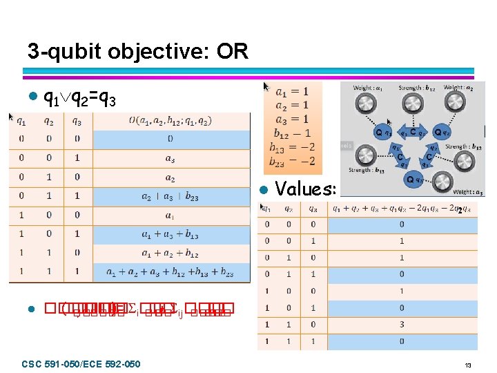
D-Wave’s Programming Model (Qubo) l OBJECTIVE: ������ Real-valued function ������ (�� : �� )= i�� �� + ij�� �� , �� ���� �� �� — minimized during annealing cycle — System samples from qi to minimize objective drive into “ground state” l l q 0 b 04 q 4 a 0 QUBIT: Quantum bit; participates in annealing cycle — settles into one of two possible final states: 0, 1 COUPLER: �� j Physical device — allows one qubit to influence another qubit WEIGHT: Real-valued constant, 1 per qubit — Influences qubit’s tendency to collapse into its 2 possible final states; controlled by the programmer STRENGTH: �� Real-valued constant, 1 per coupler — Controls influence exerted by one qubit on another; controlled by the programmer CSC 591 -050/ECE 592 -050 8

D-Wave 2 X Today — — D-Wave 2 k machine 2 k Qubits: 6 k Intra-cell couplers 8 k Inter-cell couplers — Intra: or abstract 3 D Chimera graph (L, M, N) 2 LMN L 2 MN+L(M-1)N+LM(N-1) 2 LMN+L 2 MN+L(M-1)N+LM(N-1) GC Inter: WC EC MC QC CSC 591 -050/ECE 592 -050 9

Software Environment l Accelerator (like GPU), runs quantum machine instructions (QMIs) l program qubos translate to QMIs CSC 591 -050/ECE 592 -050 10

Quantum Apprentice: 2, 3, 4 qubit simulation l See web page l your 1 st quantum pgm Later: l Connect to machine l Run there l Receive >1 answer l Interpret probability l BUT: h/w access only for IBM, not D-Wave CSC 591 -050/ECE 592 -050 11

2 -qubit objectives l Blue values minimum = objective l ������ (�� : �� )= i�� �� + ij�� �� , �� ���� �� �� CSC 591 -050/ECE 592 -050 12

3 -qubit mapping l Problem: cannot map theoretical 3 -qubo into bipartite graph l Use 2 qubit chains l l Red, yellow, green, blue chains (many adjacent placement options) Let’s start w/ 1 chain (red), only CSC 591 -050/ECE 592 -050 14

3 -qubit mapping l Problem: cannot map theoretical 3 -qubo into bipartite graph l Use 2 qubit chains l l Red, yellow, green, blue chains (many adjacent placement options) Let’s start w/ 1 chain (red), only l 4 6 neighbors CSC 591 -050/ECE 592 -050 15

Building Qubit chains l Use equal qubo b/w 2 or more qubits l causes �� 1 and 2 to be the same l Idea: if qubits differ, we’ll pay an objective penalty CSC 591 -050/ECE 592 -050 16

Embedding rules 1. 2. 3. 4. l l l A logical qubit can be mapped to N physical qubits as long as physical qubits form a connected set. We call this a chain. For each physical coupler connecting 2 physical qubits in same chain, include QUBO terms to cause the 2 physical qubits to align When a logical qubit is mapped to an N-qubit chain, divide weight for logical qubit by N & apply that weight to each qubit in chain. Split the coupling strength between two logical qubits over all available physical couplers connecting the chains corresponding to the logical qubits. q 1 Q 0 q 2 Q 4 q 3 [Q 1 Q 5] l Why does it work? CSC 591 -050/ECE 592 -050 Logical ground state = physical ground state 17

Probability Amplitudes l l Simulator: k answers (if your problem has that many answers) Quantum computer: n > k answers, each w/ probability — Here: 4 answer w/ nearly equally high probaility (rest is low) CSC 591 -050/ECE 592 -050 18

Direct Programming of D-Wave l Solver API (SAPI): for C, Matlab, python (Windows, Linux, i. OS) l Lowest level of programming l Synchronous/async. QMI instructions l Via simulation or connect to real machine (if you have access) l Choose different solvers l Advanced features — Async. Exec — Embedding — Order reduction — Spin reversal transforms — Post processing — Ising/QUBO translation CSC 591 -050/ECE 592 -050 19

SAPI Example: frustrated system l We know how to make aligned anti-aligned chains. l Combine these two chain types to build a frustrated system. CSC 591 -050/ECE 592 -050 20

QUBOs for individual constraints CSC 591 -050/ECE 592 -050 21

Aggregate QUBO l l l Confirm that QUBO represented here is sum of individual QUBOs from last slide. Input the QUBO below into Quantum Apprentice on Four Qubits tab. Confirm that you get desired set of states. — ������ =2�� 2+2�� 3− 2�� 1�� 2− 2�� 3− 2�� 3�� 4+2�� 4�� 1 Embed QUBO to unit cell — �� 0000 1⇒�� — �� 0004 2⇒�� — �� 0001 3⇒�� — �� 0005 4⇒�� Compile, run, check output CSC 591 -050/ECE 592 -050 22

Building Block: Half adder QUBO l Formulate as qubo l Requires embedding l Need ancilla bits Ø Need tool support CSC 591 -050/ECE 592 -050 23

Half Adder Derived from QUBO l Consider ground states l Find common equation (binary): x+y=s+2 c l l Convert into minimization of a QUBO — subtract RHS: x+y-s-2 c=0 x y s c ---- ---0 0 0 1 1 0 1 0 1 Transform into minimization problem — square it: (x+y-s-2 c)2 = (x+y-s-2 c) = x 2+xy-xs-2 xc+yx+y 2 -ys-2 yc-sx-sy+s 2+2 sc-2 cx-2 cy+2 cs+4 c 2= x 2+y 2+s 2+4 c 2+2 xy-2 xs-4 xc-2 ys-4 yc+4 sc — Note, for a boolean bє{0, 1}, b 2=b So we can write x+y+s+4 c+2 xy-2 xs-4 xc-2 ys-4 yc+4 sc CSC 591 -050/ECE 592 -050 24

Check Half Adder in Quantum Apprentice l l We have: x+y+s+4 c+2 xy-2 xs-4 xc-2 ys-4 yc+4 sc, same as: a 1 a 2 a 3 a 4 b 12 b 13 b 14 b 23 b 24 b 34 1 1 1 4 2 -2 -4 4 q 1 q 2 q 3 q 4 Objective 0 0 0 0 1 1 1 1 0 0 1 1 0 1 0 1 0 4 1 9 1 1 0 4 4 0 1 1 Note: another valid solution was 2 slides back CSC 591 -050/ECE 592 -050 25

Embed Half Adder l Let’s embed it: x 2+y 2+s 2+4 c 2+2 xy-2 xs-4 xc-2 ys-4 yc+4 sc — l l a 1 a 2 a 3 a 4 b 12 b 13 b 14 b 23 b 24 b 34 1 1 1 4 2 -2 -4 4 x x, x’ etc. Make sure it’s still an integer (why? ) — multiply weights/strength (here: by 2) a 1 a 2 a 3 a 4 b 12 b 13 b 14 b 23 b 24 b 34 2 2 2 8 4 -4 -8 8 Add “equal” relation with a maximal negative strength per embedding — So x, x’ need a connecting coupler with max. strength, say, -200 — x, x’ get proportional weight of 2/2+200/2=101 –Half the original wait + half the absolute value of the coupler — Same for x, y’ (optionally also s, s’ and c, c’) CSC 591 -050/ECE 592 -050 26

QMI for Half Adder l Resulting embedding (for bit 0 of x, y, s, c embedded): — x=Q 0, x’=Q 4, A 0=101, A 4=101, B 14=-200, etc. for y, s, c –b 12 C 0001 etc. — Written as QMI: C 0000 C 0 00 1 CSC 591 -050/ECE 592 -050 Q 0000 <== 101 Q 0001 <== 101 Q 0002 <== 101 … C 0000 <== -200 C 0001 <== 4 … 27

Specify Half Adder directly as QUBO l Directly specify as QUBO + embedding, then issue: #half-adder. e #half-adder. q — dw set connection laptop x 0: Q 0000 Q 0004 var: x 0 y 0: Q 0001 Q 0005 var: y 0 — dw set solver c 4 -sw_sample s 0: Q 0002 Q 0006 var: s 0 — dw mkdir –p three-bit-adder c 0: Q 0003 Q 0007 var: c 0 — dw cd three-bit-adder term: 1 * x 0 — dw embed half-adder. q half-adder. e term: 1 * y 0 term: 1 * s 0 — dw get pqmi #see QMI weights etc. term: 4 * c 0 –Embedding weight not set yet term: 2 * x 0 * y 0 — dw bind param_chain=3 term: -2 * x 0 * s 0 -4 * x 0 * c 0 –greater than max. # qubits in chain term: -2 * y 0 * s 0 term: -4 * y 0 * c 0 — dw get default. qmi #QMI code term: 4 * s 0 * c 0 — dw exec num_reads=1000 default. qmi assert: (x 0 + y 0) - (s 0 + 2*c 0) — dw val –v default. qmi #valid solutions min(objective), here 0 — dw get default. sol #see each solution CSC 591 -050/ECE 592 -050 a 1 a 2 a 3 a 4 b 12 b 13 b 14 b 23 b 24 b 34 1 1 1 4 2 -2 -4 4 28

Bias Output l Need to add a bias constraint: #half-adder. q —… param: b 0 — dw embed half-adder. q half-adder. e var: x 0 var: y 0 — dw bind param_chain=3 b 0=-1 var: s 0 –Drive s 0 1, set b 0=-1 var: c 0 –Drive s 0 0, set b 0=1 term: 1 * x 0 — dw exec num_reads=1000 default. qmi term: 1 * y 0 term: 1 * s 0 — dw get default. sol #see each solution term: 4 * c 0 –Notice: Objective=-1 for b 0=-1 !!! Term: b 0 * s 0 #half-adder. e x 0: Q 0000 Q 0004 y 0: Q 0001 Q 0005 s 0: Q 0002 Q 0006 c 0: Q 0003 Q 0007 term: 2 * x 0 * y 0 term: -2 * x 0 * s 0 term: -4 * x 0 * c 0 term: -2 * y 0 * s 0 term: -4 * y 0 * c 0 term: 4 * s 0 * c 0 assert: (x 0 + y 0) - (s 0 + 2*c 0) CSC 591 -050/ECE 592 -050 29

More complex example: 3 -bit Adder l Add two 3 -bit numbers a, b in range [0 -7] — Returns 4 -bit sum s in [0 -14] range and carry bits c (14 qbits) — 10 ancilla bits indicated by blue couplers 24 qubits total _ ~ — Notice: Embed c 0, c 0 by adding their original weights in half+full adder and then dividing by chain length: (4+1)/3 –better: find LCM(5, 3), multiply orig. weights/strength by 3&5 CSC 591 -050/ECE 592 -050 30