Quantitative Vegetation Analysis with Forest Inventory Vegetation 1

Quantitative Vegetation Analysis with Forest Inventory Vegetation 1

Outline Objective Review of Data Structures Forest inventory example dataset Species Counts Number of trees by species and plot Species presence (counts/percentages) Average number of trees per plot by species Cumulative distribution of species occurrences Frequency (histogram) of species occurrences Total number of trees per plot Number of different species Merge plot-level tables to plt table Merge species-level tables to one table Species Basal Area Basal area by species and plot Total basal area by plot Percent basal area by species and plot 2

Objective Of This Lesson ## Learn tools in R for quantitative analyses of forest inventory vegetation data. These tools will help you get acquainted with your vegetation dataset and prepare you for multivariate analyses of vegetation species and modeling species distributions. # Explore tree data. # Summarize tree data to plot-level. # Species abundance (Evenness) - the total number of trees sampled, by species (by plot). - the average number of trees sampled per plot. - percent plots a species occurs on. # Species richness (Diversity) - the number of different species per plot. - cumulative number of different species within sampled population. # Graphically display tree data. # Histograms - distributions of univariate tree data (binned into categories). # Barplots - distributions of tree data by specified category. 3

Multivariate Statistics ## Packages and Links for R and multivariate statistics R Package – vegan (Jari Oksanen) Contains tools for analyzing ecological communities, including species analyses and multivariate analyses. • Diversity indices • Species richness and abundance models • Ordination R Package – labdsv (Dave Roberts) Includes tutorials and lab exercises for a course in quantitative analysis and multivariate statistics in vegetation ecology • Modeling species distributions • Ordination techniques • Cluster analysis Link to package on CRAN website http: //cran. r-project. org/web/packages/vegan/index. html This document explains diversity related methods in vegan. http: //cran. r-project. org/web/packages/vegan/vignettes/diversity-vegan. pdf R Labs for Vegetation Ecologists - Tutorial using vegan package (Dave Roberts; Montana State University) 4 http: //ecology. msu. montana. edu/labdsv/R/labs/

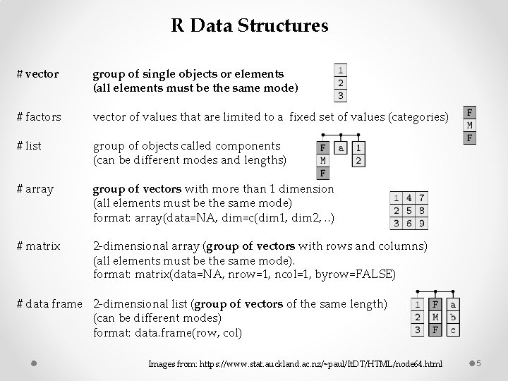
R Data Structures # vector group of single objects or elements (all elements must be the same mode) # factors vector of values that are limited to a fixed set of values (categories) # list group of objects called components (can be different modes and lengths) # array group of vectors with more than 1 dimension (all elements must be the same mode) format: array(data=NA, dim=c(dim 1, dim 2, . . ) # matrix 2 -dimensional array (group of vectors with rows and columns) (all elements must be the same mode). format: matrix(data=NA, nrow=1, ncol=1, byrow=FALSE) # data frame 2 -dimensional list (group of vectors of the same length) (can be different modes) format: data. frame(row, col) Images from: https: //www. stat. auckland. ac. nz/~paul/It. DT/HTML/node 64. html 5

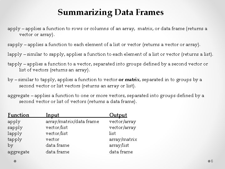
Summarizing Data Frames apply – applies a function to rows or columns of an array, matrix, or data frame (returns a vector or array). sapply – applies a function to each element of a list or vector (returns a vector or array). lapply – similar to sapply, applies a function to each element of a list or vector (returns a list). tapply – applies a function to a vector, separated into groups defined by a second vector or list of vectors (returns an array). by – similar to tapply, applies a function to vector or matrix, separated in to groups by a second vector or list vectors (returns an array or list). aggregate – applies a function to one or more vectors, separated into groups defined by a second vector or list of vectors (returns a data frame). Function apply sapply lapply tapply by aggregate Input array/matrix/data frame vector/list vector data frame Output vector/array list array/matrix array/list data frame 6

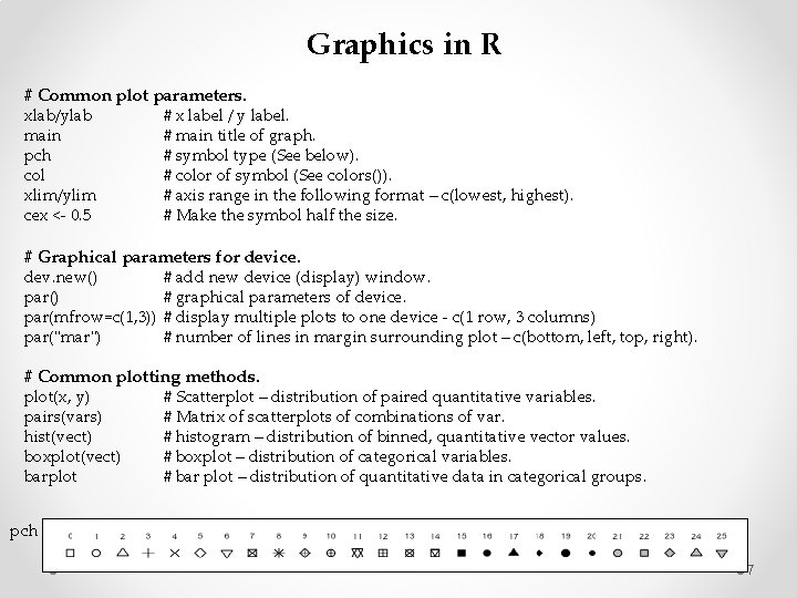
Graphics in R # Common plot parameters. xlab/ylab main pch col xlim/ylim cex <- 0. 5 # x label / y label. # main title of graph. # symbol type (See below). # color of symbol (See colors()). # axis range in the following format – c(lowest, highest). # Make the symbol half the size. # Graphical parameters for device. dev. new() par(mfrow=c(1, 3)) par("mar") # add new device (display) window. # graphical parameters of device. # display multiple plots to one device - c(1 row, 3 columns) # number of lines in margin surrounding plot – c(bottom, left, top, right). # Common plotting methods. plot(x, y) pairs(vars) hist(vect) boxplot(vect) barplot # Scatterplot – distribution of paired quantitative variables. # Matrix of scatterplots of combinations of var. # histogram – distribution of binned, quantitative vector values. # boxplot – distribution of categorical variables. # bar plot – distribution of quantitative data in categorical groups. pch 7

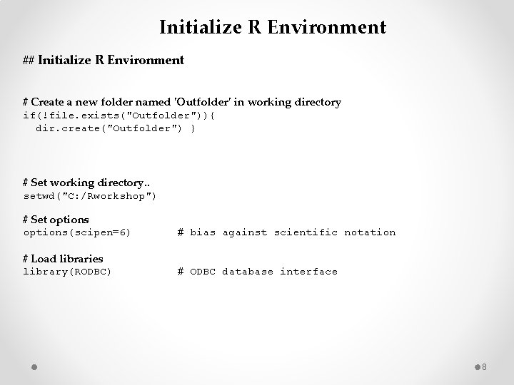
Initialize R Environment ## Initialize R Environment # Create a new folder named 'Outfolder' in working directory if(!file. exists("Outfolder")){ dir. create("Outfolder") } # Set working directory. . setwd("C: /Rworkshop") # Set options(scipen=6) # bias against scientific notation # Load libraries library(RODBC) # ODBC database interface 8

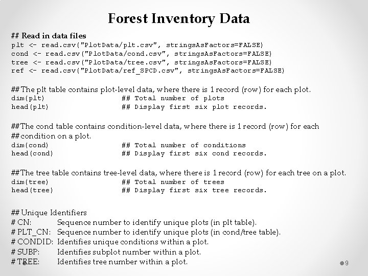
Forest Inventory Data ## Read in data files plt <- read. csv("Plot. Data/plt. csv", strings. As. Factors=FALSE) cond <- read. csv("Plot. Data/cond. csv", strings. As. Factors=FALSE) tree <- read. csv("Plot. Data/tree. csv", strings. As. Factors=FALSE) ref <- read. csv("Plot. Data/ref_SPCD. csv", strings. As. Factors=FALSE) ## The plt table contains plot-level data, where there is 1 record (row) for each plot. dim(plt) head(plt) ## Total number of plots ## Display first six plot records. ## The cond table contains condition-level data, where there is 1 record (row) for each ## condition on a plot. dim(cond) head(cond) ## Total number of conditions ## Display first six cond records. ## The tree table contains tree-level data, where there is 1 record (row) for each tree on a plot. dim(tree) head(tree) ## Total number of trees ## Display first six tree records. ## Unique Identifiers # CN: Sequence number to identify unique plots (in plt table). # PLT_CN: Sequence number to identify unique plots (in cond/tree table). # CONDID: Identifies unique conditions within a plot. # SUBP: Identifies subplot number within a plot. # TREE: Identifies tree number within a plot. 9

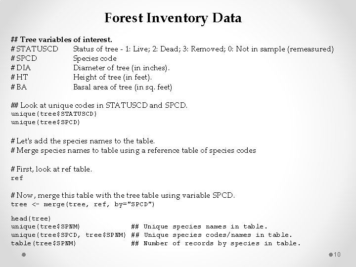
Forest Inventory Data ## Tree variables of interest. # STATUSCD Status of tree - 1: Live; 2: Dead; 3: Removed; 0: Not in sample (remeasured) # SPCD Species code # DIA Diameter of tree (in inches). # HT Height of tree (in feet). # BA Basal area of tree (in sq. feet) ## Look at unique codes in STATUSCD and SPCD. unique(tree$STATUSCD) unique(tree$SPCD) # Let's add the species names to the table. # Merge species names to table using a reference table of species codes # First, look at ref table. ref # Now, merge this table with the tree table using variable SPCD. tree <- merge(tree, ref, by="SPCD") head(tree) unique(tree$SPNM) ## Unique species names in table. unique(tree$SPCD, tree$SPNM) ## Unique species codes/names in table(tree$SPNM) ## Number of records by species in table. 10

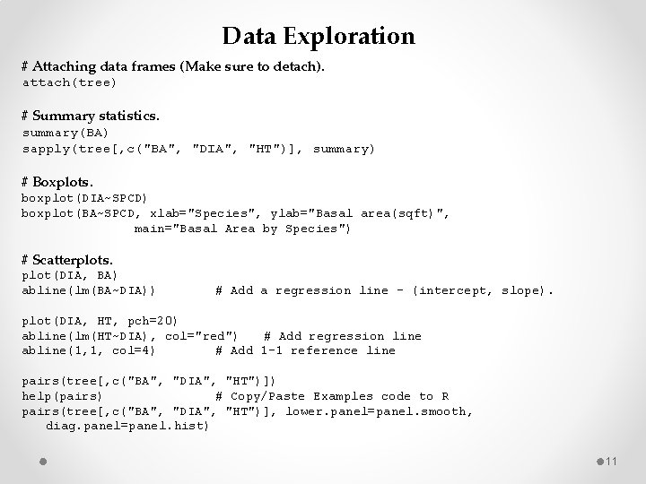
Data Exploration # Attaching data frames (Make sure to detach). attach(tree) # Summary statistics. summary(BA) sapply(tree[, c("BA", "DIA", "HT")], summary) # Boxplots. boxplot(DIA~SPCD) boxplot(BA~SPCD, xlab="Species", ylab="Basal area(sqft)", main="Basal Area by Species") # Scatterplots. plot(DIA, BA) abline(lm(BA~DIA)) # Add a regression line - (intercept, slope). plot(DIA, HT, pch=20) abline(lm(HT~DIA), col="red") # Add regression line abline(1, 1, col=4) # Add 1 -1 reference line pairs(tree[, c("BA", "DIA", "HT")]) help(pairs) # Copy/Paste Examples code to R pairs(tree[, c("BA", "DIA", "HT")], lower. panel=panel. smooth, diag. panel=panel. hist) 11

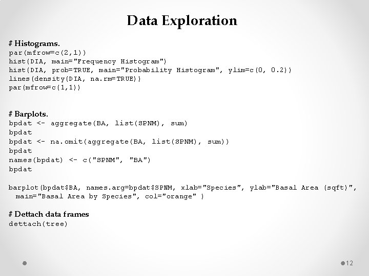
Data Exploration # Histograms. par(mfrow=c(2, 1)) hist(DIA, main="Frequency Histogram") hist(DIA, prob=TRUE, main="Probability Histogram", ylim=c(0, 0. 2)) lines(density(DIA, na. rm=TRUE)) par(mfrow=c(1, 1)) # Barplots. bpdat <- aggregate(BA, list(SPNM), sum) bpdat <- na. omit(aggregate(BA, list(SPNM), sum)) bpdat names(bpdat) <- c("SPNM", "BA") bpdat barplot(bpdat$BA, names. arg=bpdat$SPNM, xlab="Species", ylab="Basal Area (sqft)", main="Basal Area by Species", col="orange" ) # Dettach data frames dettach(tree) 12

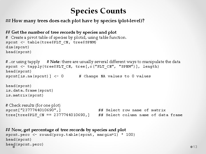
Species Counts ## How many trees does each plot have by species (plot-level)? ## Get the number of tree records by species and plot # Create a pivot table of species by plotid, using table function. spcnt <- table(tree$PLT_CN, tree$SPNM) dim(spcnt) head(spcnt) #. . or using tapply # Note: there are usually several different ways to manipulate the data spcnt <- tapply(tree$PLT_CN, tree[, c("PLT_CN", "SPNM")], length) head(spcnt) spcnt[is. na(spcnt)] <- 0 # Change NA values to 0 values head(spcnt) is. data. frame(spcnt) is. matrix(spcnt) # Check results (for one plot) spcnt["2377744010690", ] tree[tree$PLT_CN == 2377744010690, ] ## Select row name of matrix ## Select column name of data frame ## Now, get percentage of tree records by species and plot spcnt. perc <- round(prop. table(spcnt, margin=1) * 100) head(spcnt. perc) 13

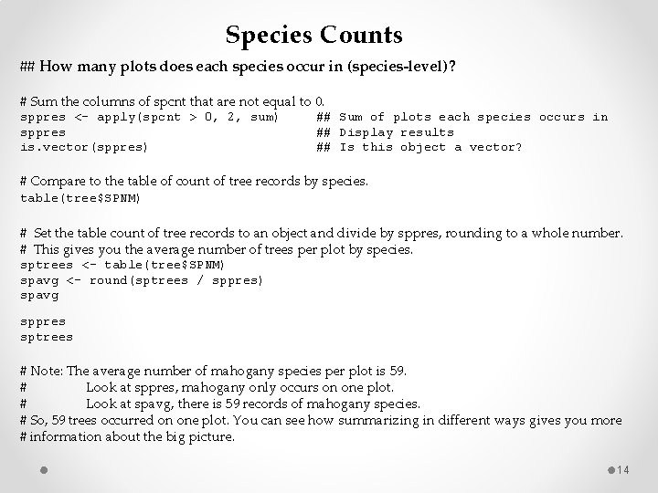
Species Counts ## How many plots does each species occur in (species-level)? # Sum the columns of spcnt that are not equal to 0. sppres <- apply(spcnt > 0, 2, sum) sppres is. vector(sppres) ## Sum of plots each species occurs in ## Display results ## Is this object a vector? # Compare to the table of count of tree records by species. table(tree$SPNM) # Set the table count of tree records to an object and divide by sppres, rounding to a whole number. # This gives you the average number of trees per plot by species. sptrees <- table(tree$SPNM) spavg <- round(sptrees / sppres) spavg sppres sptrees # Note: The average number of mahogany species per plot is 59. # Look at sppres, mahogany only occurs on one plot. # Look at spavg, there is 59 records of mahogany species. # So, 59 trees occurred on one plot. You can see how summarizing in different ways gives you more # information about the big picture. 14

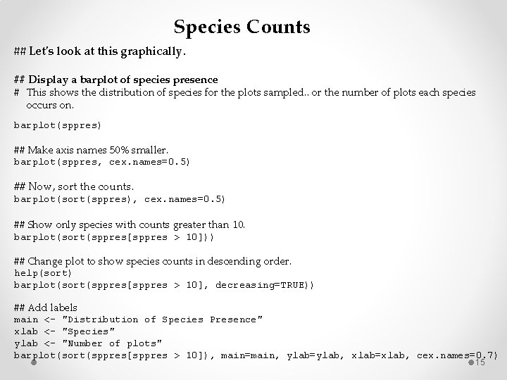
Species Counts ## Let's look at this graphically. ## Display a barplot of species presence # This shows the distribution of species for the plots sampled. . or the number of plots each species occurs on. barplot(sppres) ## Make axis names 50% smaller. barplot(sppres, cex. names=0. 5) ## Now, sort the counts. barplot(sort(sppres), cex. names=0. 5) ## Show only species with counts greater than 10. barplot(sort(sppres[sppres > 10])) ## Change plot to show species counts in descending order. help(sort) barplot(sort(sppres[sppres > 10], decreasing=TRUE)) ## Add labels main <- "Distribution of Species Presence" xlab <- "Species" ylab <- "Number of plots" barplot(sort(sppres[sppres > 10]), main=main, ylab=ylab, xlab=xlab, cex. names=0. 7) 15

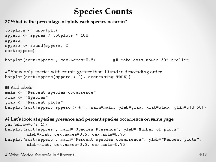
Species Counts ## What is the percentage of plots each species occur in? totplots <- nrow(plt) spperc <- sppres / totplots * 100 spperc <- round(spperc, 2) sort(spperc) barplot(sort(spperc), cex. names=0. 5) ## Make axis names 50% smaller ## Show only species with counts greater than 10 and in descending order barplot(sort(spperc[spperc > 4], decreasing=TRUE)) ## Add labels main <- "Percent species occurrence" xlab <- "Species" ylab <- "Percent plots" barplot(sort(spperc[spperc > 4]), main=main, ylab=ylab, xlab=xlab, ylim=c(0, 50)) ## Let's look at species presence and percent species occurrence on same page par(mfrow=c(2, 1)) barplot(sort(sppres), main="Species Presence", ylab="Number of plots", xlab=xlab, cex. names=0. 5, cex. axis=0. 75) barplot(sort(spperc), main="Percent species occurrence", ylab="Percent plots", xlab=xlab, cex. names=0. 5, cex. axis=0. 75) # Note: Notice the scale is different. 16

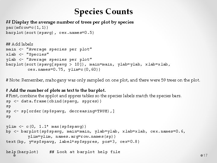
Species Counts ## Display the average number of trees per plot by species par(mfrow=c(1, 1)) barplot(sort(spavg), cex. names=0. 5) ## Add labels main <- "Average species xlab <- "Species" ylab <- "Average species barplot(sort(spavg[spavg cex. names=0. 75, per plot" > 10]), main=main, ylab=ylab, xlab=xlab, ylim=c(0, 60)) # Note: Remember, mahogany was only sampled on one plot, and there were 59 trees on the plot. # Add the number of plots as text to the bar plot. # First, combine the spplot and sppres tables so the species labels match the species bars. sp <- data. frame(cbind(spavg, sppres)) sp sp <- sp[order(sp$spavg, decreasing=TRUE), ] sp ylim <- c(0, 1. 1* max(sp$spavg)) bp <- barplot(sp$spavg, main=main, ylab=ylab, xlab=xlab, cex. names=0. 6, ylim=ylim, names. arg=row. names(sp)) text(bp, y=sp$spavg, label=sp$sppres, pos=3, cex=0. 8) help(barplot) ## Look at barplot help file 17

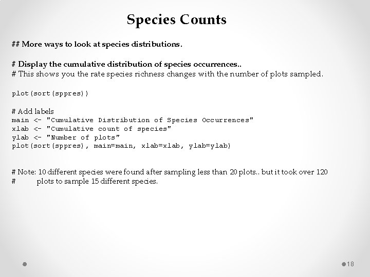
Species Counts ## More ways to look at species distributions. # Display the cumulative distribution of species occurrences. . # This shows you the rate species richness changes with the number of plots sampled. plot(sort(sppres)) # Add labels main <- "Cumulative Distribution of Species Occurrences" xlab <- "Cumulative count of species" ylab <- "Number of plots" plot(sort(sppres), main=main, xlab=xlab, ylab=ylab) # Note: 10 different species were found after sampling less than 20 plots. . but it took over 120 # plots to sample 15 different species. 18

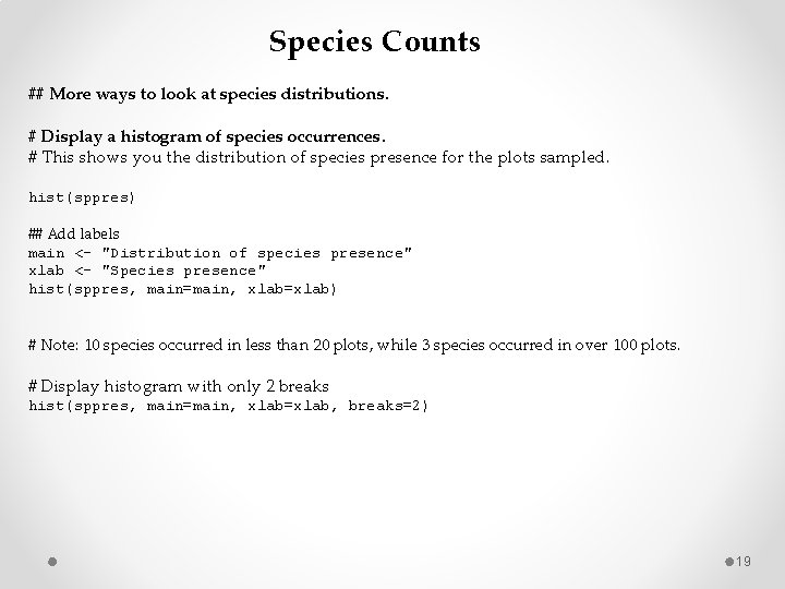
Species Counts ## More ways to look at species distributions. # Display a histogram of species occurrences. # This shows you the distribution of species presence for the plots sampled. hist(sppres) ## Add labels main <- "Distribution of species presence" xlab <- "Species presence" hist(sppres, main=main, xlab=xlab) # Note: 10 species occurred in less than 20 plots, while 3 species occurred in over 100 plots. # Display histogram with only 2 breaks hist(sppres, main=main, xlab=xlab, breaks=2) 19

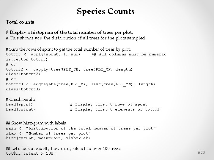
Species Counts Total counts # Display a histogram of the total number of trees per plot. # This shows you the distribution of all trees for the plots sampled. # Sum the rows of spcnt to get the total number of trees by plot. totcnt <- apply(spcnt, 1, sum) ## All columns must be numeric is. vector(totcnt) # or totcnt 2 <- tapply(tree$PLT_CN, length) class(totcnt 2) # or totcnt 3 <- aggregate(tree$PLT_CN, list(tree$PLT_CN), length) class(totcnt 3) # Check results head(spcnt) head(totcnt) # Display first 6 rows of spcnt # Display first 6 elements of totcnt ## Show histogram with labels main <- "Distribution of the total number of trees per plot" xlab <- "Number of trees per plot" hist(totcnt, main=main, xlab=xlab) ## Let's look at exactly how many plots had over 100 trees. totcnt[totcnt > 100] 20

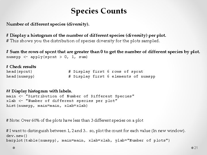
Species Counts Number of different species (diversity). # Display a histogram of the number of different species (diversity) per plot. # This shows you the distribution of species diversity for the plots sampled. # Sum the rows of spcnt that are greater than 0 to get the number of different species by plot. numspp <- apply(spcnt > 0, 1, sum) # Check results head(spcnt) head(numspp) # Display first 6 rows of spcnt # Display first 6 elements of numspp ## Display histogram with labels. main <- "Distribution of Number of Different Species" xlab <- "Number of different species per plot" hist(numspp, main=main, xlab=xlab) # Note: Over 60% of the plots have less than 3 different species on a plot # I want to distinguish between 1, 2 and 3. . so, plot the count for each value (In new window). dev. new() barplot(table(numspp), main=main, xlab=xlab, ylab="Number of plots") 21

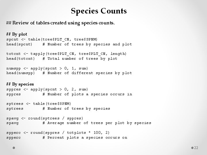
Species Counts ## Review of tables created using species counts. ## By plot spcnt <- table(tree$PLT_CN, tree$SPNM) head(spcnt) # Number of trees by species and plot totcnt <- tapply(tree$PLT_CN, length) head(totcnt) # Total number of trees by plot numspp <- apply(spcnt > 0, 1, sum) head(numspp) # Number of different species by plot ## By species sppres <- apply(spcnt > 0, 2, sum) sppres # Number of plots a species occurs in sptrees <- table(tree$SPNM) sptrees # Number of trees by species spavg <- round(sptrees / sppres) spavg # Average number of trees per plot by species spperc <- round(sppres / totplots * 100, 2) spperc # Percent plots a species occurs on 22

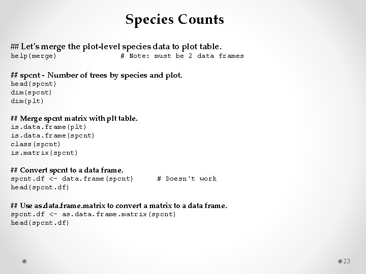
Species Counts ## Let's merge the plot-level species data to plot table. help(merge) # Note: must be 2 data frames ## spcnt - Number of trees by species and plot. head(spcnt) dim(plt) ## Merge spcnt matrix with plt table. is. data. frame(plt) is. data. frame(spcnt) class(spcnt) is. matrix(spcnt) ## Convert spcnt to a data frame. spcnt. df <- data. frame(spcnt) head(spcnt. df) # Doesn't work ## Use as. data. frame. matrix to convert a matrix to a data frame. spcnt. df <- as. data. frame. matrix(spcnt) head(spcnt. df) 23

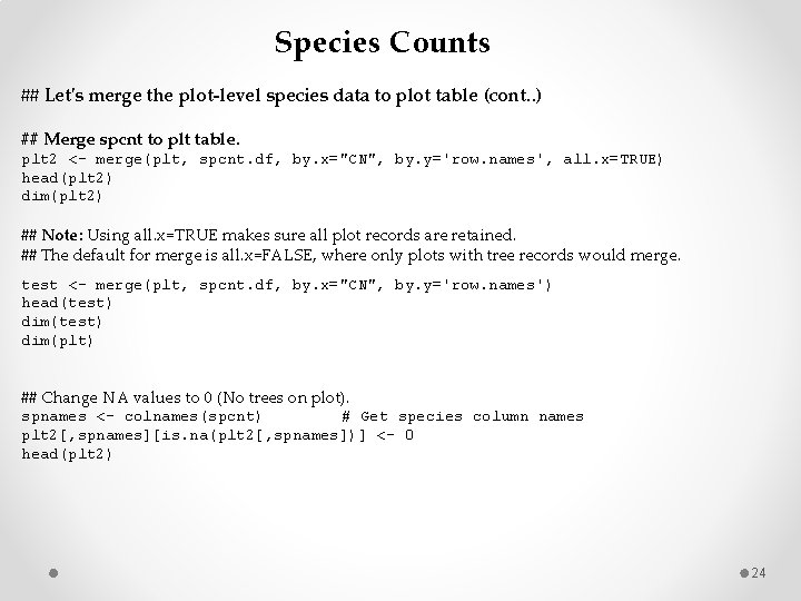
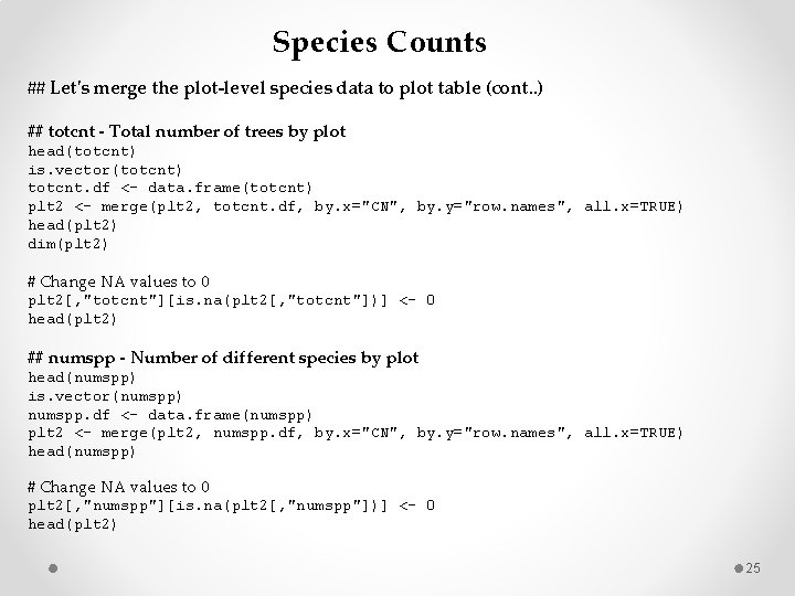
Species Counts ## Let's merge the plot-level species data to plot table (cont. . ) ## Merge spcnt to plt table. plt 2 <- merge(plt, spcnt. df, by. x="CN", by. y='row. names', all. x=TRUE) head(plt 2) dim(plt 2) ## Note: Using all. x=TRUE makes sure all plot records are retained. ## The default for merge is all. x=FALSE, where only plots with tree records would merge. test <- merge(plt, spcnt. df, by. x="CN", by. y='row. names') head(test) dim(plt) ## Change NA values to 0 (No trees on plot). spnames <- colnames(spcnt) # Get species column names plt 2[, spnames][is. na(plt 2[, spnames])] <- 0 head(plt 2) 24

Species Counts ## Let's merge the plot-level species data to plot table (cont. . ) ## totcnt - Total number of trees by plot head(totcnt) is. vector(totcnt) totcnt. df <- data. frame(totcnt) plt 2 <- merge(plt 2, totcnt. df, by. x="CN", by. y="row. names", all. x=TRUE) head(plt 2) dim(plt 2) # Change NA values to 0 plt 2[, "totcnt"][is. na(plt 2[, "totcnt"])] <- 0 head(plt 2) ## numspp - Number of different species by plot head(numspp) is. vector(numspp) numspp. df <- data. frame(numspp) plt 2 <- merge(plt 2, numspp. df, by. x="CN", by. y="row. names", all. x=TRUE) head(numspp) # Change NA values to 0 plt 2[, "numspp"][is. na(plt 2[, "numspp"])] <- 0 head(plt 2) 25

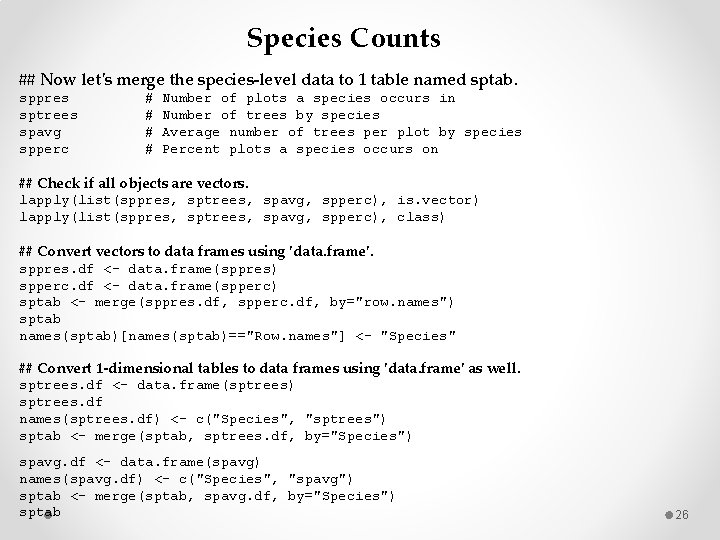
Species Counts ## Now let's merge the species-level data to 1 table named sptab. sppres sptrees spavg spperc # # Number of plots a species occurs in Number of trees by species Average number of trees per plot by species Percent plots a species occurs on ## Check if all objects are vectors. lapply(list(sppres, sptrees, spavg, spperc), is. vector) lapply(list(sppres, sptrees, spavg, spperc), class) ## Convert vectors to data frames using 'data. frame'. sppres. df <- data. frame(sppres) spperc. df <- data. frame(spperc) sptab <- merge(sppres. df, spperc. df, by="row. names") sptab names(sptab)[names(sptab)=="Row. names"] <- "Species" ## Convert 1 -dimensional tables to data frames using 'data. frame' as well. sptrees. df <- data. frame(sptrees) sptrees. df names(sptrees. df) <- c("Species", "sptrees") sptab <- merge(sptab, sptrees. df, by="Species") spavg. df <- data. frame(spavg) names(spavg. df) <- c("Species", "spavg") sptab <- merge(sptab, spavg. df, by="Species") sptab 26

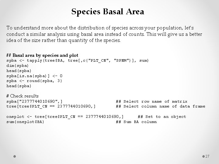
Species Basal Area To understand more about the distribution of species across your population, let's conduct a similar analysis using basal area instead of counts. This will give us a better idea of the size rather than quantity of the species. ## Basal area by species and plot spba <- tapply(tree$BA, tree[, c("PLT_CN", "SPNM")], sum) dim(spba) head(spba) spba[is. na(spba)] <- 0 spba <- round(spba, 3) head(spba) # Check results spba["2377744010690", ] tree[tree$PLT_CN == 2377744010690, ] ## Select row name of matrix ## Select column name of data frame oneplot <- tree[tree$PLT_CN == 2377744010690, ] ## Set to an object sum(oneplot$BA) ## Sum BA column 27

Species Basal Area ## Total basal area by plot. totba <- tapply(tree$BA, tree[, "PLT_CN"], sum) totba ## Let's round the totba values to 2 decimal points. totba <- round(totba, 2) ## Check the total basal area for oneplot totba[names(totba) == unique(oneplot$PLT_CN)] sum(oneplot$BA) ## Percent basal area by species and plot spbaperc <- round((spba / as. vector(totba)) * 100, 2) head(spbaperc) # or spbaperc 2 <- round(prop. table(spba, margin=1) * 100, 2) head(spbaperc 2) # Check results spbaperc["2378381010690", ] spba["2378381010690", ] totba["2378381010690"] 28

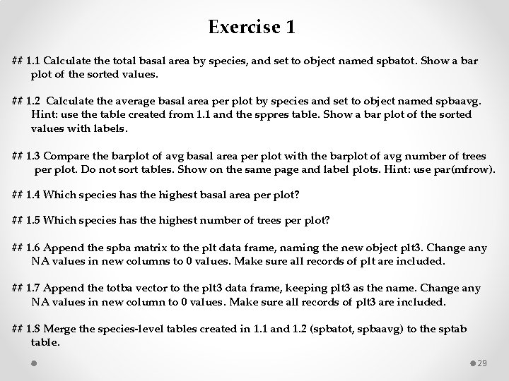
Exercise 1 ## 1. 1 Calculate the total basal area by species, and set to object named spbatot. Show a bar plot of the sorted values. ## 1. 2 Calculate the average basal area per plot by species and set to object named spbaavg. Hint: use the table created from 1. 1 and the sppres table. Show a bar plot of the sorted values with labels. ## 1. 3 Compare the barplot of avg basal area per plot with the barplot of avg number of trees per plot. Do not sort tables. Show on the same page and label plots. Hint: use par(mfrow). ## 1. 4 Which species has the highest basal area per plot? ## 1. 5 Which species has the highest number of trees per plot? ## 1. 6 Append the spba matrix to the plt data frame, naming the new object plt 3. Change any NA values in new columns to 0 values. Make sure all records of plt are included. ## 1. 7 Append the totba vector to the plt 3 data frame, keeping plt 3 as the name. Change any NA values in new column to 0 values. Make sure all records of plt 3 are included. ## 1. 8 Merge the species-level tables created in 1. 1 and 1. 2 (spbatot, spbaavg) to the sptab table. 29