Quantitative Methods Varsha Varde Quantitative Methods Quantifying Uncertainty

Quantitative Methods Varsha Varde

Quantitative Methods Quantifying Uncertainty: Basic Concepts of Probability

Quotes from You and Me • Chances of your getting a handsome job should improve if you obtain an MBA. • Probably, collections will jump this month. • Most probably, ERP will be on by June. • Odds are great for my promotion this time. • Winning cricket match against Australia is not impossible, but is highly improbable Defects from new machines are unlikely. Varsha Varde 3

Uncertainty • • • Each Statement Involves Uncertainty. Chances = Odds = Likelihood = Probability Real Life is Usually Full of Uncertainty. Almost Nothing is for Sure. There are Chances of Something Happening and Chances of Something Else Happening. • In Such Situations, You can’t ‘Prove’ Anything. • All You Can Do is to Assign a Probability to Each of the Different Possible Outcomes. Varsha Varde 4

Quotes from You and Me After This MBA • Chances of your getting a handsome job would be 90% if you obtain an MBA. • I am 75% confident that collections will jump this month. • Odds are 80: 20 for my promotion this time. • . Winning cricket match against Australia is not impossible but has only 10% chance • New machines churn out good product 97 out of 100 times. Varsha Varde 5

Probability Theory • How Do You Say 90% Chances, or 80: 20 Odds, or 75% Confidence? • Probability Theory Provides Tools to Decision Makers to Quantify Uncertainties. Varsha Varde 6

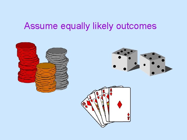
Assigning Probabilities • Classical Approach: Assumes equally likely outcomes (card games , dice games, tossing coins and the like) • Relative Frequency Approach: Uses relative frequencies of past occurrences as probabilities (Decision problems in area of management. Delay in delivery of product) • Subjective Approach : Guess based on past experience or intuition. ( At higher level of managerial decisions for important , specific and unique decisions

Assume equally likely outcomes

Use Relative Frequencies • Making use of relative frequencies of past. • Suppose an organisation knows from past data that about 25 out of 300 employees entering every year leave due to good opportunities elsewhere • then the organisation can predict the probability of employee turnover for this reason • as 25/300=1/12=0. 083

Subjective Probability • Based on personal judgements • Uses individual’s experience and familiarity with facts • An expert analyst of share prices may give his judgement as follows on price of ACC shares in next two months • 20% probability of increase by Rs 500 or more • 60% probability of increase by less than Rs 500 • 20%probability of remaining unchanged

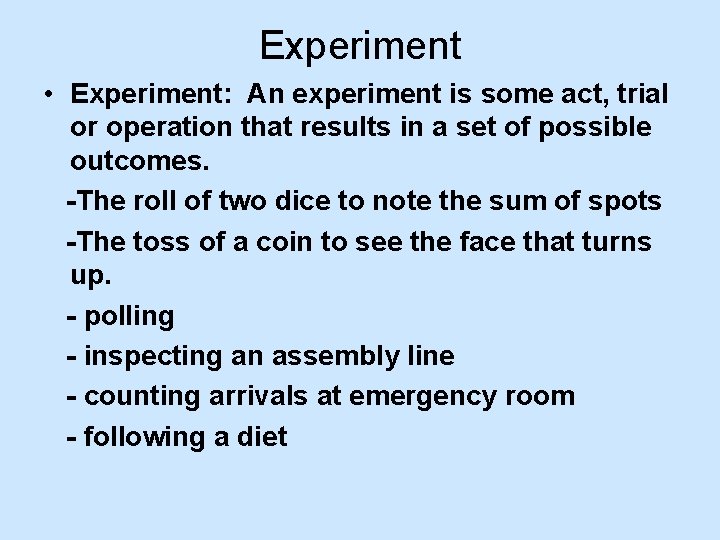
Experiment • Experiment: An experiment is some act, trial or operation that results in a set of possible outcomes. -The roll of two dice to note the sum of spots -The toss of a coin to see the face that turns up. - polling - inspecting an assembly line - counting arrivals at emergency room - following a diet

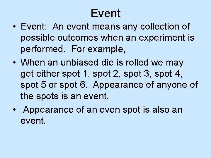
Event • Event: An event means any collection of possible outcomes when an experiment is performed. For example, • When an unbiased die is rolled we may get either spot 1, spot 2, spot 3, spot 4, spot 5 or spot 6. Appearance of anyone of the spots is an event. • Appearance of an even spot is also an event.

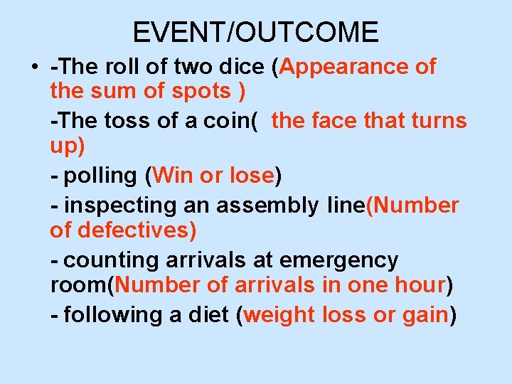
EVENT/OUTCOME • -The roll of two dice (Appearance of the sum of spots ) -The toss of a coin( the face that turns up) - polling (Win or lose) - inspecting an assembly line(Number of defectives) - counting arrivals at emergency room(Number of arrivals in one hour) - following a diet (weight loss or gain)

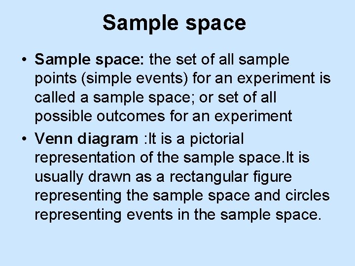
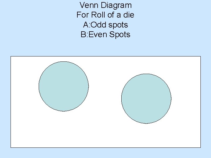
Sample space • Sample space: the set of all sample points (simple events) for an experiment is called a sample space; or set of all possible outcomes for an experiment • Venn diagram : It is a pictorial representation of the sample space. It is usually drawn as a rectangular figure representing the sample space and circles representing events in the sample space.

Venn Diagram For Roll of a die A: Odd spots B: Even Spots

Equally Likely Events • Equiprobable or Equally Likely Events: Events are said to be equiprobable when one does not occur more often than the others. • When an unbiased die is thrown any one of the six spots may appear. • When an unbiased coin is tossed either a head or a tail appears

Exhaustive Events • Exhaustive Events: Events are said to be exhaustive when they include all possible cases or outcomes. For example, in tossing of fair coin, the two events “appearance of a head” and “appearance of a tail” are exhaustive events because when a coin is tossed we would get either a head or a tail.

Independent Events • Independent Events: Two events A and B are said to be independent if occurrence of A does not affect and is not affected by the occurrence of B. • When a coin is tossed twice the result of the first toss does not affect and is not affected by the result of the second toss. Thus, the result of the first toss and the result of the second toss are independent events.

Dependent Events • Dependent Events: Two events A and B are called dependent if the occurrence of A affects or is affected by the occurrence of B. • For example, there are four kings in a pack of 52 cards. The event of drawing a king at the first draw and the event of drawing another king at the second draw when the first drawn king is not replaced, are two dependent events. In the first event there are four kings in a pack of 52 cards and in the second event there are only three kings left in the pack of remaining 51 cards

Mutually Exclusive Events • Events are termed mutually exclusive if they cannot occur together so that in any one trial of an experiment at most one of the events would occur. • Mutually Exclusive Events: • “throwing even” and “throwing odd” with one die, • “drawing the spade, ” “drawing a diamond” and “drawing a club” while drawing one card from a deck. • purchase of a machine out of 3 brands available • Not mutually exclusive • “drawing a spade” and “drawing a queen” • “even number” and “at least 3” with one die • Selection of a candidate with post graduate qualification and over 3 years experience • A particular easy way to obtain two mutually exclusive events is to consider an event and its negative(Complement). Such as “even” and “not even, ” “spade”, “not spade” or in general ‘A’ and ‘not A’.

Notation. • Sample space : S • Sample point: E 1, E 2, . . . etc. • Event: A, B, C, D, E etc. (any capital letter). • Venn diagram: Example. • S = {E 1, E 2, . . . , E 6}. • That is S = {1, 2, 3, 4, 5, 6}. We may think of S as representation of possible outcomes of a throw of a die. Varsha Varde 21

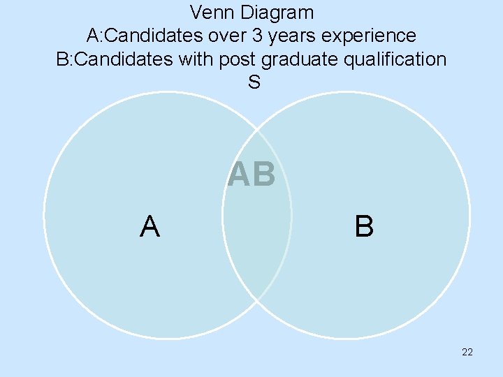
Venn Diagram A: Candidates over 3 years experience B: Candidates with post graduate qualification S AB A B 22

More definitions • Union, Intersection and Complementation Given A and B two events in a sample space S. 1. The union of A and B, AUB, is the event containing all sample points in either A or B or both. Sometimes we use A or B for union. 2. The intersection of A and B, A∩B, is the event containing all sample points that are both in A and B. Sometimes we use AB or A and B for intersection. 3. The complement of A, Ā the event containing all sample points that are not in A. Sometimes we use not A or Ac for complement. Mutually Exclusive Events (Disjoint Events) 4 Two events are said to be mutually exclusive (or disjoint) if their intersection is empty. (i. e. A ∩ B = ö). Varsha Varde 23

Example • • Suppose S = {E 1, E 2, . . . , E 6}. Let A = {E 1, E 3, E 5}; B = {E 1, E 2, E 3}. Then (i)A U B = {E 1, E 2, E 3, E 5}. (ii) A ∩ B = {E 1, E 3}. (iii) Ā = {E 2, E 4, E 6}; Bc ={E 4, E 5, E 6}; (iv) A and B are not mutually exclusive (why? ) • (v) Give two events in S that are mutually exclusive. Varsha Varde 24

Probability of an event • Relative Frequency Definition If an experiment is repeated a large number, n, of times and the event A is observed n. A times, the probability of A is • P(A) = n. A / n • Interpretation • n = # of trials of an experiment • n. A = frequency of the event A • n. A/n = relative frequency of A • P(A) = n. A /n , if n is large enough. Varsha Varde 25

Basic Formula of Probability • Probability of an Event A: No. of Outcomes Favourable to Event A = --------------------------Total Number of All Possible Outcomes • Probability is a Ratio. (A Distribution Ratio) It varies from 0 to 1. • Often, It is Expressed in Percentage Terms Ranging from 0% to 100%. • It is denoted as P(A) and termed as marginal or unconditional probability Varsha Varde 26

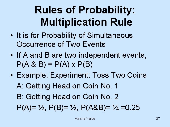
Rules of Probability: Multiplication Rule • It is for Probability of Simultaneous Occurrence of Two Events • If A and B are two independent events, P(A & B) = P(A) x P(B) • Example: Experiment: Toss Two Coins A: Getting Head on Coin No. 1 B: Getting Head on Coin No. 2 P(A)= ½, P(B)= ½, P(A&B)= ¼ =0. 25 Varsha Varde 27

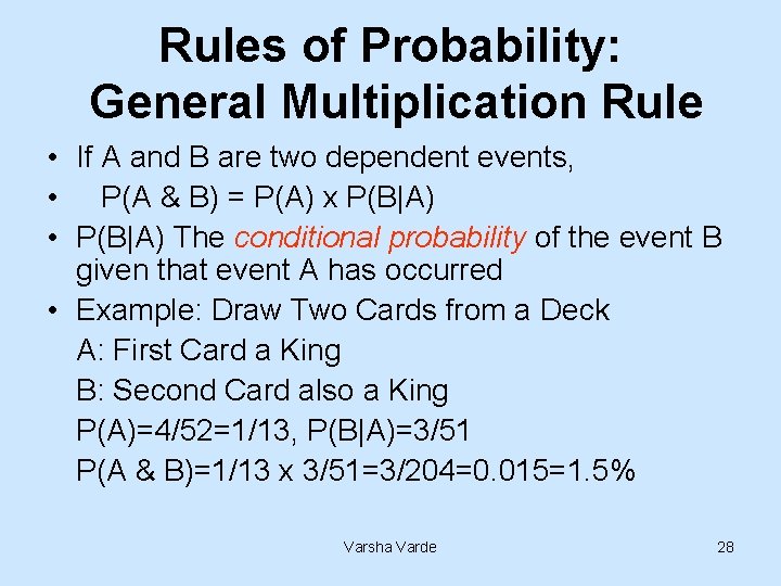
Rules of Probability: General Multiplication Rule • If A and B are two dependent events, • P(A & B) = P(A) x P(B|A) • P(B|A) The conditional probability of the event B given that event A has occurred • Example: Draw Two Cards from a Deck A: First Card a King B: Second Card also a King P(A)=4/52=1/13, P(B|A)=3/51 P(A & B)=1/13 x 3/51=3/204=0. 015=1. 5% Varsha Varde 28

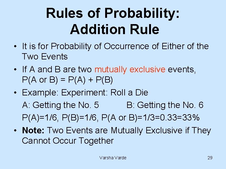
Rules of Probability: Addition Rule • It is for Probability of Occurrence of Either of the Two Events • If A and B are two mutually exclusive events, P(A or B) = P(A) + P(B) • Example: Experiment: Roll a Die A: Getting the No. 5 B: Getting the No. 6 P(A)=1/6, P(B)=1/6, P(A or B)=1/3=0. 33=33% • Note: Two Events are Mutually Exclusive if They Cannot Occur Together Varsha Varde 29

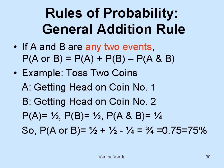
Rules of Probability: General Addition Rule • If A and B are any two events, P(A or B) = P(A) + P(B) – P(A & B) • Example: Toss Two Coins A: Getting Head on Coin No. 1 B: Getting Head on Coin No. 2 P(A)= ½, P(B)= ½, P(A & B)= ¼ So, P(A or B)= ½ + ½ - ¼ = ¾ =0. 75=75% Varsha Varde 30

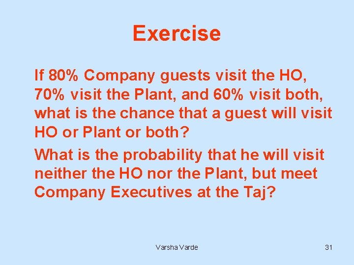
Exercise If 80% Company guests visit the HO, 70% visit the Plant, and 60% visit both, what is the chance that a guest will visit HO or Plant or both? What is the probability that he will visit neither the HO nor the Plant, but meet Company Executives at the Taj? Varsha Varde 31

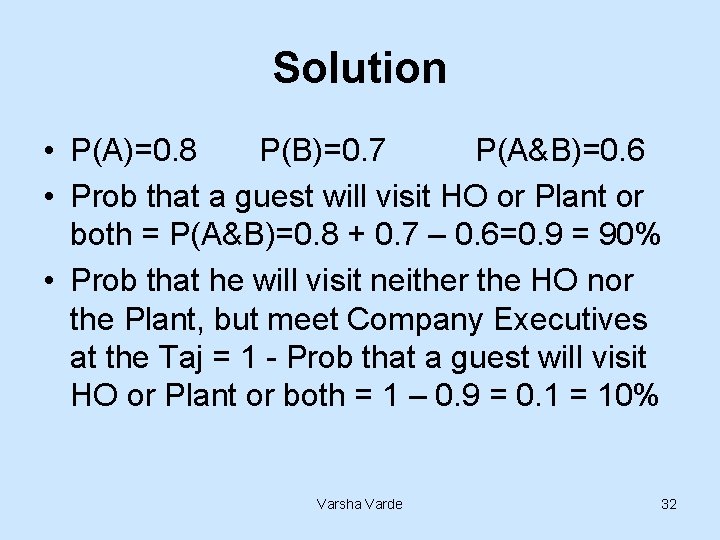
Solution • P(A)=0. 8 P(B)=0. 7 P(A&B)=0. 6 • Prob that a guest will visit HO or Plant or both = P(A&B)=0. 8 + 0. 7 – 0. 6=0. 9 = 90% • Prob that he will visit neither the HO nor the Plant, but meet Company Executives at the Taj = 1 - Prob that a guest will visit HO or Plant or both = 1 – 0. 9 = 0. 1 = 10% Varsha Varde 32

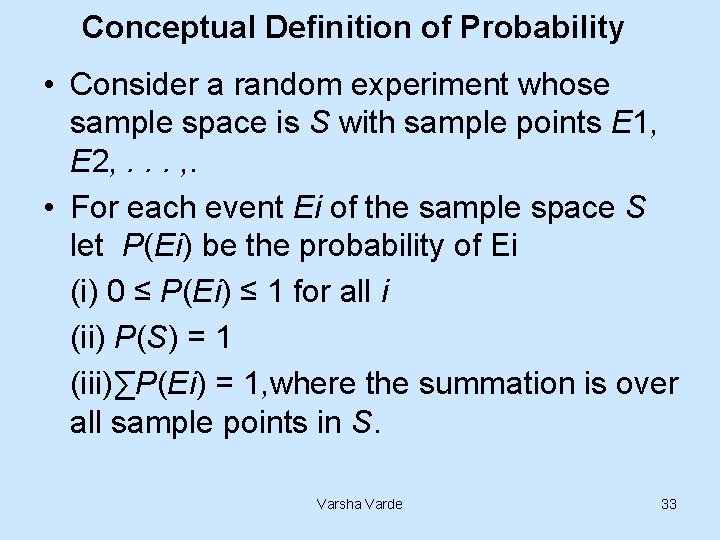
Conceptual Definition of Probability • Consider a random experiment whose sample space is S with sample points E 1, E 2, . . . , . • For each event Ei of the sample space S let P(Ei) be the probability of Ei (i) 0 ≤ P(Ei) ≤ 1 for all i (ii) P(S) = 1 (iii)∑P(Ei) = 1, where the summation is over all sample points in S. Varsha Varde 33

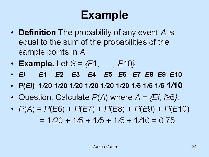
Example • Definition The probability of any event A is equal to the sum of the probabilities of the sample points in A. • Example. Let S = {E 1, . . . , E 10}. • Ei E 1 E 2 E 3 E 4 E 5 E 6 E 7 E 8 E 9 E 10 • P(Ei) 1/20 1/20 1/5 1/5 1/10 • Question: Calculate P(A) where A = {Ei, i≥ 6}. • P(A) = P(E 6) + P(E 7) + P(E 8) + P(E 9) + P(E 10) = 1/20 + 1/5 + 1/10 = 0. 75 Varsha Varde 34

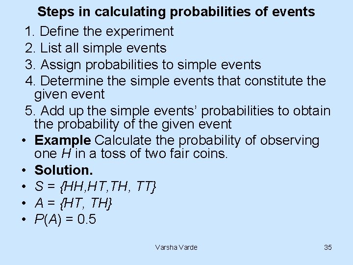
Steps in calculating probabilities of events 1. Define the experiment 2. List all simple events 3. Assign probabilities to simple events 4. Determine the simple events that constitute the given event 5. Add up the simple events’ probabilities to obtain the probability of the given event • Example Calculate the probability of observing one H in a toss of two fair coins. • Solution. • S = {HH, HT, TH, TT} • A = {HT, TH} • P(A) = 0. 5 Varsha Varde 35

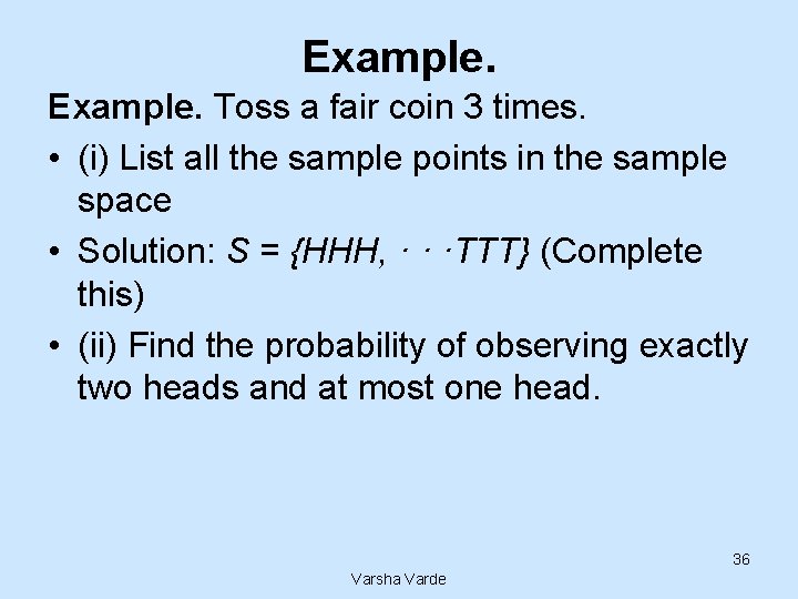
Example. Toss a fair coin 3 times. • (i) List all the sample points in the sample space • Solution: S = {HHH, · · ·TTT} (Complete this) • (ii) Find the probability of observing exactly two heads and at most one head. 36 Varsha Varde

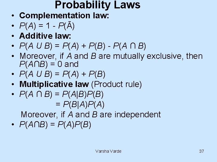
• • • Probability Laws Complementation law: P(A) = 1 - P(Ā) Additive law: P(A U B) = P(A) + P(B) - P(A ∩ B) Moreover, if A and B are mutually exclusive, then P(A∩B) = 0 and P(A U B) = P(A) + P(B) Multiplicative law (Product rule) P(A ∩ B) = P(A|B)P(B) = P(B|A)P(A) Moreover, if A and B are independent P(A∩B) = P(A)P(B) Varsha Varde 37

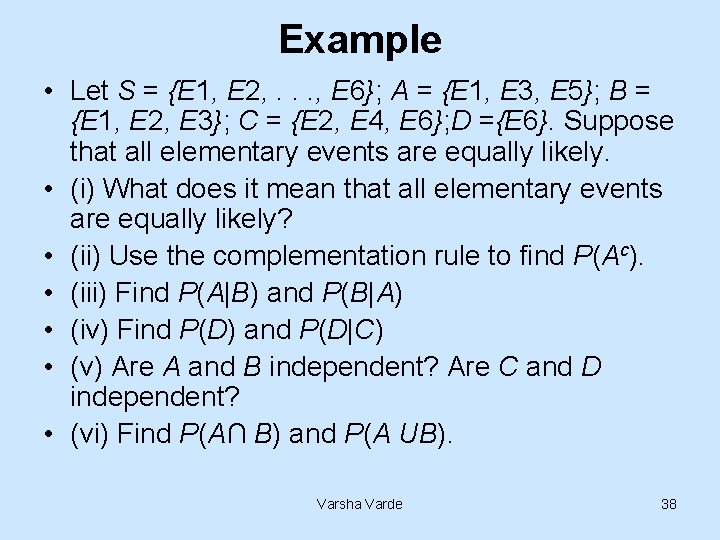
Example • Let S = {E 1, E 2, . . . , E 6}; A = {E 1, E 3, E 5}; B = {E 1, E 2, E 3}; C = {E 2, E 4, E 6}; D ={E 6}. Suppose that all elementary events are equally likely. • (i) What does it mean that all elementary events are equally likely? • (ii) Use the complementation rule to find P(Ac). • (iii) Find P(A|B) and P(B|A) • (iv) Find P(D) and P(D|C) • (v) Are A and B independent? Are C and D independent? • (vi) Find P(A∩ B) and P(A UB). Varsha Varde 38

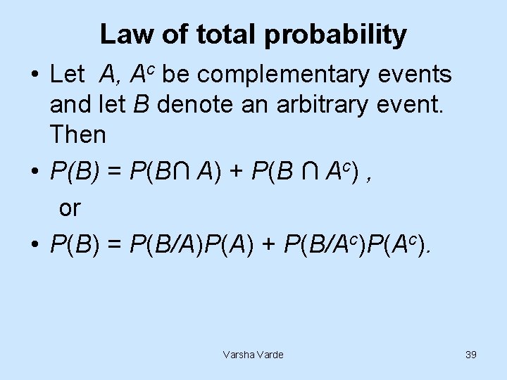
Law of total probability • Let A, Ac be complementary events and let B denote an arbitrary event. Then • P(B) = P(B∩ A) + P(B ∩ Ac) , or • P(B) = P(B/A)P(A) + P(B/Ac)P(Ac). Varsha Varde 39

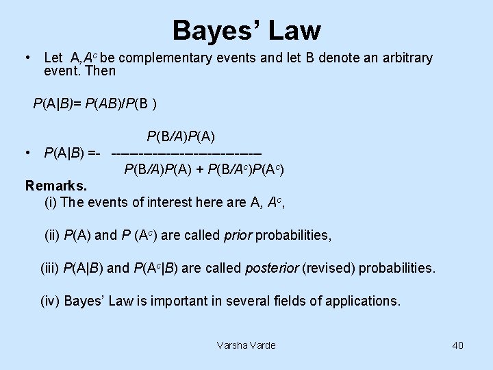
Bayes’ Law • Let A, Ac be complementary events and let B denote an arbitrary event. Then P(A|B)= P(AB)/P(B ) P(B/A)P(A) • P(A|B) =- ----------------P(B/A)P(A) + P(B/Ac)P(Ac) Remarks. (i) The events of interest here are A, Ac, (ii) P(A) and P (Ac) are called prior probabilities, (iii) P(A|B) and P(Ac|B) are called posterior (revised) probabilities. (iv) Bayes’ Law is important in several fields of applications. Varsha Varde 40

Bayesian Approach English mathematician Thomas Bayes (1702 -61) set out his theory of probability It is being revived now 250 years later Step ahead from Subjective Prob Method

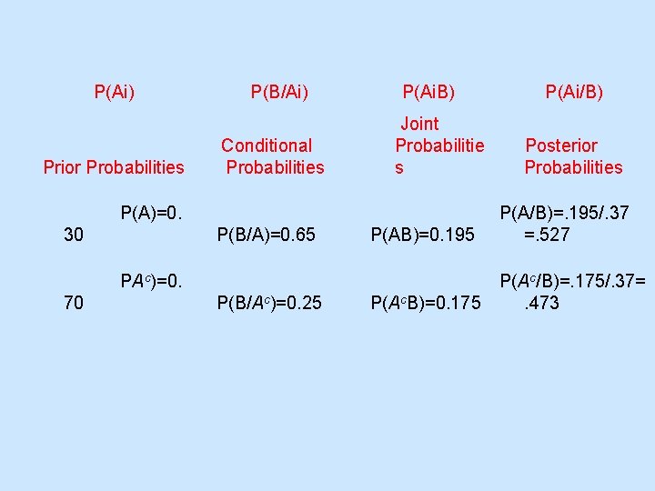
P(Ai) Prior Probabilities P(B/Ai) Conditional Probabilities P(Ai. B) Joint Probabilitie s P(A)=0. 30 P(B/A)=0. 65 P(B/Ac)=0. 25 Posterior Probabilities P(AB)=0. 195 P(A/B)=. 195/. 37 =. 527 P(Ac. B)=0. 175 P(Ac/B)=. 175/. 37=. 473 PAc)=0. 70 P(Ai/B)

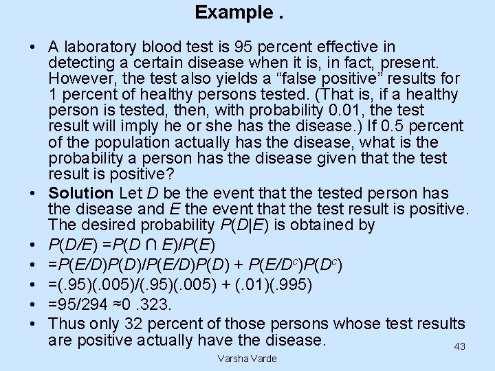
Example. • A laboratory blood test is 95 percent effective in detecting a certain disease when it is, in fact, present. However, the test also yields a “false positive” results for 1 percent of healthy persons tested. (That is, if a healthy person is tested, then, with probability 0. 01, the test result will imply he or she has the disease. ) If 0. 5 percent of the population actually has the disease, what is the probability a person has the disease given that the test result is positive? • Solution Let D be the event that the tested person has the disease and E the event that the test result is positive. The desired probability P(D|E) is obtained by • P(D/E) =P(D ∩ E)/P(E) • =P(E/D)P(D)/P(E/D)P(D) + P(E/Dc)P(Dc) • =(. 95)(. 005)/(. 95)(. 005) + (. 01)(. 995) • =95/294 ≈0. 323. • Thus only 32 percent of those persons whose test results are positive actually have the disease. 43 Varsha Varde

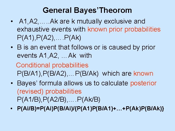
General Bayes’Theorom • A 1, A 2, …. . Ak are k mutually exclusive and exhaustive events with known prior probabilities P(A 1), P(A 2), …. P(Ak) • B is an event that follows or is caused by prior events A 1, A 2, …Ak with Conditional probabilities P(B/A 1), P(B/A 2), …P(B/Ak) which are known • Bayes’ formula allows us to calculate posterior (revised) probabilities P(A 1/B), P(A 2/B), …. P(Ak/B) • P(Ai/B)=P(Ai)P(B/Ai)/{P(A 1)P(B/A 1)+…+P(Ak)P(B/Ak)}

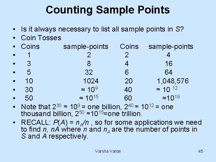
Counting Sample Points • • • Is it always necessary to list all sample points in S? Coin Tosses Coins sample-points 1 2 2 4 3 8 4 16 5 32 6 64 10 1024 20 1, 048, 576 30 ≈ 109 40 ≈ 10 12 50 ≈ 1015 60 ≈1019 Note that 230 ≈ 109 = one billion, 240 ≈ 1012 = one thousand billion, 250 ≈1015=one trillion. • RECALL: P(A) = n. A/n , so for some applications we need to find n, n. A where n and n. A are the number of points in S and A respectively. Varsha Varde 45

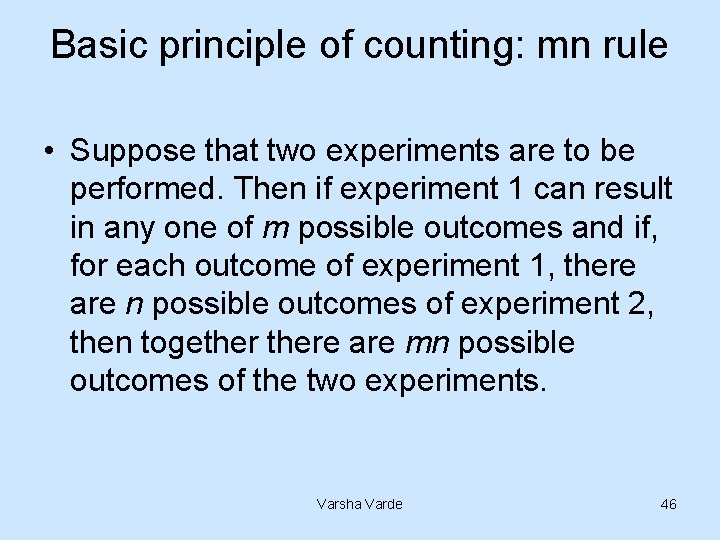
Basic principle of counting: mn rule • Suppose that two experiments are to be performed. Then if experiment 1 can result in any one of m possible outcomes and if, for each outcome of experiment 1, there are n possible outcomes of experiment 2, then togethere are mn possible outcomes of the two experiments. Varsha Varde 46

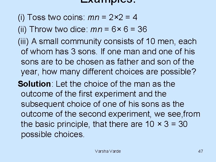
Examples. (i) Toss two coins: mn = 2× 2 = 4 (ii) Throw two dice: mn = 6× 6 = 36 (iii) A small community consists of 10 men, each of whom has 3 sons. If one man and one of his sons are to be chosen as father and son of the year, how many different choices are possible? Solution: Let the choice of the man as the outcome of the first experiment and the subsequent choice of one of his sons as the outcome of the second experiment, we see, from the basic principle, that there are 10 × 3 = 30 possible choices. Varsha Varde 47

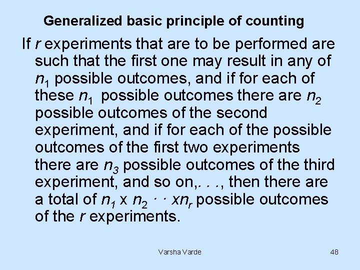
Generalized basic principle of counting If r experiments that are to be performed are such that the first one may result in any of n 1 possible outcomes, and if for each of these n 1 possible outcomes there are n 2 possible outcomes of the second experiment, and if for each of the possible outcomes of the first two experiments there are n 3 possible outcomes of the third experiment, and so on, . . . , then there a total of n 1 x n 2 · · xnr possible outcomes of the r experiments. Varsha Varde 48

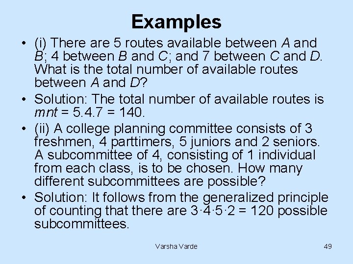
Examples • (i) There are 5 routes available between A and B; 4 between B and C; and 7 between C and D. What is the total number of available routes between A and D? • Solution: The total number of available routes is mnt = 5. 4. 7 = 140. • (ii) A college planning committee consists of 3 freshmen, 4 parttimers, 5 juniors and 2 seniors. A subcommittee of 4, consisting of 1 individual from each class, is to be chosen. How many different subcommittees are possible? • Solution: It follows from the generalized principle of counting that there are 3· 4· 5· 2 = 120 possible subcommittees. Varsha Varde 49

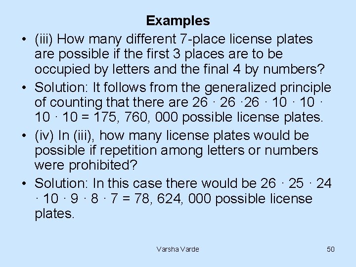
• • Examples (iii) How many different 7 -place license plates are possible if the first 3 places are to be occupied by letters and the final 4 by numbers? Solution: It follows from the generalized principle of counting that there are 26 · 10 · 10 = 175, 760, 000 possible license plates. (iv) In (iii), how many license plates would be possible if repetition among letters or numbers were prohibited? Solution: In this case there would be 26 · 25 · 24 · 10 · 9 · 8 · 7 = 78, 624, 000 possible license plates. Varsha Varde 50

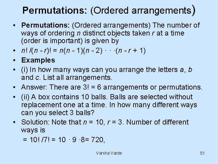
Permutations: (Ordered arrangements) • Permutations: (Ordered arrangements) The number of ways of ordering n distinct objects taken r at a time (order is important) is given by • n! /(n - r)! = n(n - 1)(n - 2) · · ·(n - r + 1) • Examples • (i) In how many ways can you arrange the letters a, b and c. List all arrangements. • Answer: There are 3! = 6 arrangements or permutations. • (ii) A box contains 10 balls. Balls are selected without replacement one at a time. In how many different ways can you select 3 balls? • Solution: Note that n = 10, r = 3. Number of different ways is = 10! /7! = 10 · 9 · 8= 720, Varsha Varde 51

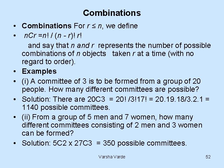
Combinations • Combinations For r ≤ n, we define • n. Cr =n! / (n - r)! r! and say that n and r represents the number of possible combinations of n objects taken r at a time (with no regard to order). • Examples • (i) A committee of 3 is to be formed from a group of 20 people. How many different committees are possible? • Solution: There are 20 C 3 = 20! /3!17! = 20. 19. 18/3. 2. 1 = 1140 possible committees. • (ii) From a group of 5 men and 7 women, how many different committees consisting of 2 men and 3 women can be formed? • Solution: 5 C 2 x 27 C 3 = 350 possible committees. Varsha Varde 52

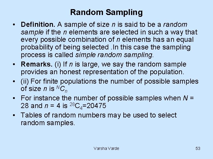
Random Sampling • Definition. A sample of size n is said to be a random sample if the n elements are selected in such a way that every possible combination of n elements has an equal probability of being selected. In this case the sampling process is called simple random sampling. • Remarks. (i) If n is large, we say the random sample provides an honest representation of the population. • (ii) For finite populations the number of possible samples of size n is NCn • For instance the number of possible samples when N = 28 and n = 4 is 28 C 4=20475 • Tables of random numbers may be used to select random samples. Varsha Varde 53

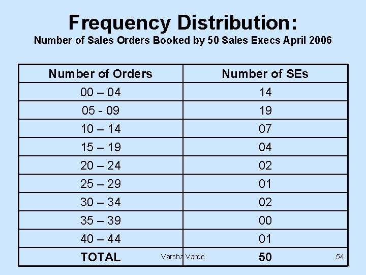
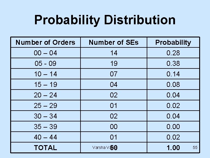
Frequency Distribution: Number of Sales Orders Booked by 50 Sales Execs April 2006 Number of Orders 00 – 04 05 - 09 10 – 14 Number of SEs 14 19 07 15 – 19 20 – 24 25 – 29 30 – 34 35 – 39 40 – 44 TOTAL 04 02 01 02 00 01 50 Varsha Varde 54

Probability Distribution Number of Orders 00 – 04 05 - 09 10 – 14 15 – 19 20 – 24 25 – 29 30 – 34 35 – 39 40 – 44 TOTAL Number of SEs 14 19 07 04 02 01 02 00 01 Varsha Varde 50 Probability 0. 28 0. 38 0. 14 0. 08 0. 04 0. 02 0. 04 0. 00 0. 02 1. 00 55

Standard Discrete Prob Distns • Binomial Distribution: When a Situation can have Only Two Possible Outcomes e. g. PASS or FAIL, ACCEPT or REJECT. • This distribution gives probability of an outcome (say, ACCEPT) occurring exactly m times out of n trials of the situation, i. e. probability of 10 ACCEPTANCES out of 15 items tested. Varsha Varde 56

Standard Discrete Prob Distns • Poisson Distribution: When a Situation can have Only Two Possible Outcomes, & When the Total Number of Observations is Large (>20), Unknown or Innumerable. • This distribution gives the probability of an outcome (say, ACCEPT) occurring m times, i. e. probability of say 150 ACCEPTANCES. Varsha Varde 57

Standard Continuous Prob Distn • Normal Distribution: Useful & Important • Several Variables Follow Normal Distn or a Pattern Nearing It. (Weights, Heights) • Skewed Distns Assume This Shape After Getting Rid of Outliers • For Large No. of Observations, Discrete Distributions Tend to Follow Normal Distn • It is Amenable to Mathematical Processes Varsha Varde 58

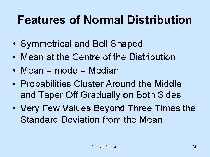
Features of Normal Distribution • • Symmetrical and Bell Shaped Mean at the Centre of the Distribution Mean = mode = Median Probabilities Cluster Around the Middle and Taper Off Gradually on Both Sides • Very Few Values Beyond Three Times the Standard Deviation from the Mean Varsha Varde 59

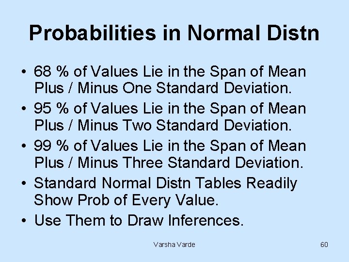
Probabilities in Normal Distn • 68 % of Values Lie in the Span of Mean Plus / Minus One Standard Deviation. • 95 % of Values Lie in the Span of Mean Plus / Minus Two Standard Deviation. • 99 % of Values Lie in the Span of Mean Plus / Minus Three Standard Deviation. • Standard Normal Distn Tables Readily Show Prob of Every Value. • Use Them to Draw Inferences. Varsha Varde 60