QUANTITATIVE METHODS 1 SAMIR K SRIVASTAVA Quantitative Methods

QUANTITATIVE METHODS 1 SAMIR K. SRIVASTAVA Quantitative Methods 1

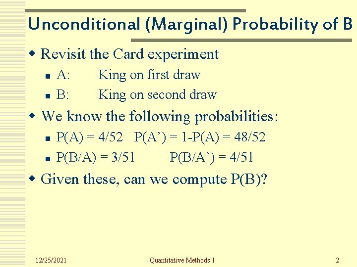
Unconditional (Marginal) Probability of B w Revisit the Card experiment n n A: B: King on first draw King on second draw w We know the following probabilities: n n P(A) = 4/52 P(A’) = 1 -P(A) = 48/52 P(B/A) = 3/51 P(B/A’) = 4/51 w Given these, can we compute P(B)? 12/25/2021 Quantitative Methods 1 2

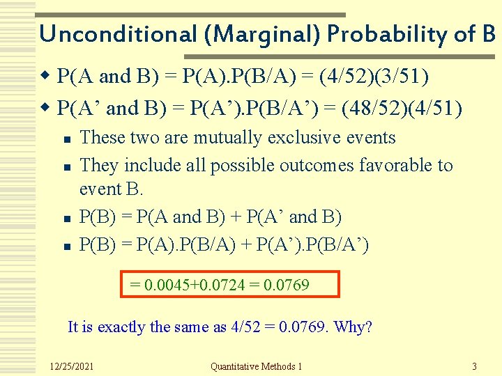
Unconditional (Marginal) Probability of B w P(A and B) = P(A). P(B/A) = (4/52)(3/51) w P(A’ and B) = P(A’). P(B/A’) = (48/52)(4/51) n n These two are mutually exclusive events They include all possible outcomes favorable to event B. P(B) = P(A and B) + P(A’ and B) P(B) = P(A). P(B/A) + P(A’). P(B/A’) = 0. 0045+0. 0724 = 0. 0769 It is exactly the same as 4/52 = 0. 0769. Why? 12/25/2021 Quantitative Methods 1 3

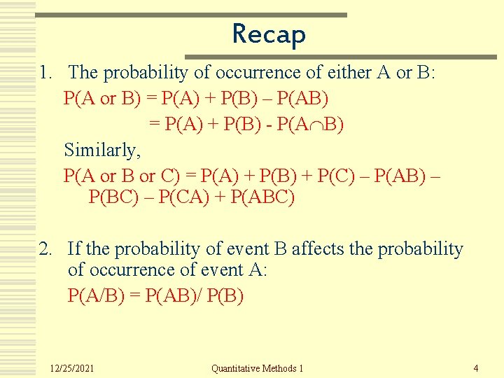
Recap 1. The probability of occurrence of either A or B: P(A or B) = P(A) + P(B) – P(AB) = P(A) + P(B) - P(A B) Similarly, P(A or B or C) = P(A) + P(B) + P(C) – P(AB) – P(BC) – P(CA) + P(ABC) 2. If the probability of event B affects the probability of occurrence of event A: P(A/B) = P(AB)/ P(B) 12/25/2021 Quantitative Methods 1 4

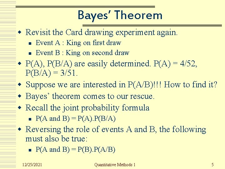
Bayes’ Theorem w Revisit the Card drawing experiment again. n n Event A : King on first draw Event B : King on second draw w P(A), P(B/A) are easily determined. P(A) = 4/52, P(B/A) = 3/51. w Suppose we are interested in P(A/B)!!! How to find it? w Bayes’ theorem comes to our rescue. w Recall the joint probability formula n P(A and B) = P(A). P(B/A) w Reversing the role of events A and B, the following must also be true: n P(A and B) = P(B). P(A/B) 12/25/2021 Quantitative Methods 1 5

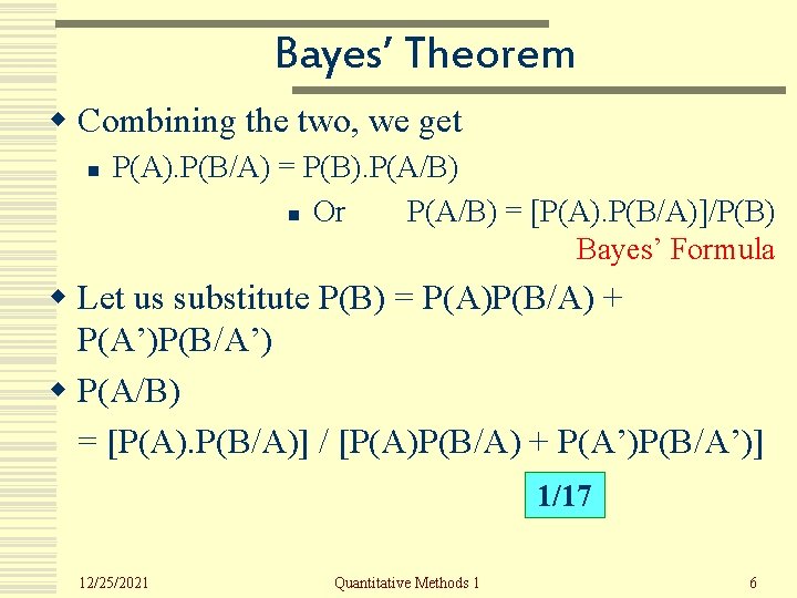
Bayes’ Theorem w Combining the two, we get n P(A). P(B/A) = P(B). P(A/B) n Or P(A/B) = [P(A). P(B/A)]/P(B) Bayes’ Formula w Let us substitute P(B) = P(A)P(B/A) + P(A’)P(B/A’) w P(A/B) = [P(A). P(B/A)] / [P(A)P(B/A) + P(A’)P(B/A’)] 1/17 12/25/2021 Quantitative Methods 1 6

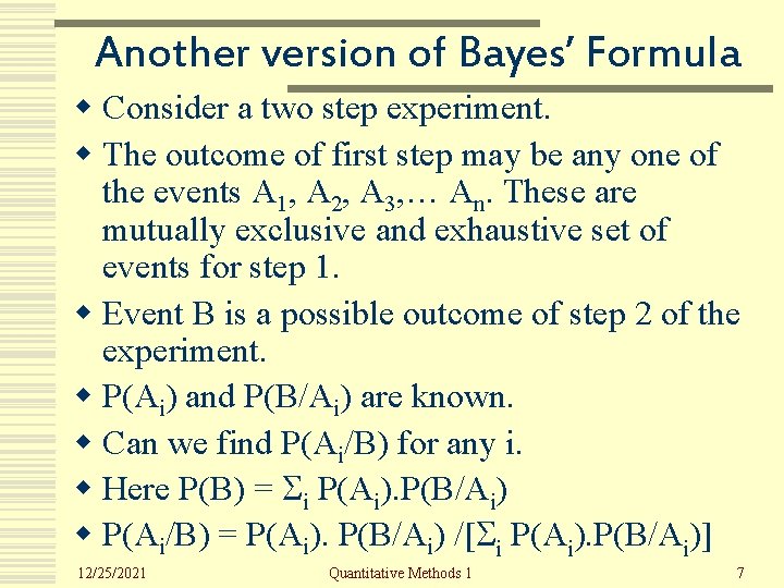
Another version of Bayes’ Formula w Consider a two step experiment. w The outcome of first step may be any one of the events A 1, A 2, A 3, … An. These are mutually exclusive and exhaustive set of events for step 1. w Event B is a possible outcome of step 2 of the experiment. w P(Ai) and P(B/Ai) are known. w Can we find P(Ai/B) for any i. w Here P(B) = i P(Ai). P(B/Ai) w P(Ai/B) = P(Ai). P(B/Ai) /[ i P(Ai). P(B/Ai)] 12/25/2021 Quantitative Methods 1 7

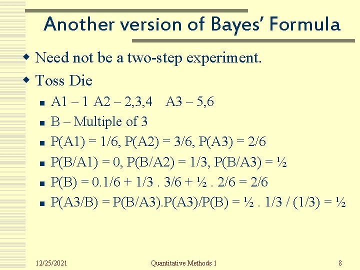
Another version of Bayes’ Formula w Need not be a two-step experiment. w Toss Die n n n A 1 – 1 A 2 – 2, 3, 4 A 3 – 5, 6 B – Multiple of 3 P(A 1) = 1/6, P(A 2) = 3/6, P(A 3) = 2/6 P(B/A 1) = 0, P(B/A 2) = 1/3, P(B/A 3) = ½ P(B) = 0. 1/6 + 1/3. 3/6 + ½. 2/6 = 2/6 P(A 3/B) = P(B/A 3). P(A 3)/P(B) = ½. 1/3 / (1/3) = ½ 12/25/2021 Quantitative Methods 1 8

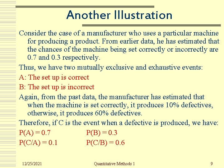
Another Illustration Consider the case of a manufacturer who uses a particular machine for producing a product. From earlier data, he has estimated that the chances of the machine being set correctly or incorrectly are 0. 7 and 0. 3 respectively. Thus, we have two mutually exclusive and exhaustive events: A: The set up is correct B: The set up is incorrect Again, from the past data, the manufacturer has estimated that when the machine is set correctly, it produces 10% defectives, otherwise, it produces 60% defectives. Therefore, if C is the event when a defective is produced, we have: P(A) = 0. 7 P(B) = 0. 3 P(C/A) = 0. 1 P(C/B) = 0. 6 12/25/2021 Quantitative Methods 1 9

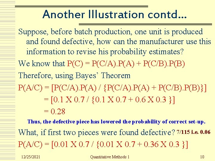
Another Illustration contd… Suppose, before batch production, one unit is produced and found defective, how can the manufacturer use this information to revise his probability estimates? We know that P(C) = P(C/A). P(A) + P(C/B). P(B) Therefore, using Bayes’ Theorem P(A/C) = [P(C/A). P(A) / {P(C/A). P(A) + P(C/B). P(B)}] = [0. 1 X 0. 7 / {0. 1 X 0. 7 + 0. 6 X 0. 3 }] = 0. 28 Thus, the defective piece has lowered the probability of correct set-up. What, if first two pieces were found defective? 7/115 i. e. 0. 06 P(A/C) = [0. 01 X 0. 7 / {0. 01 X 0. 7 + 0. 36 X 0. 3 }] 12/25/2021 Quantitative Methods 1 10

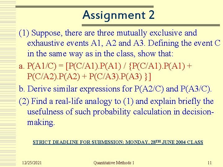
Assignment 2 (1) Suppose, there are three mutually exclusive and exhaustive events A 1, A 2 and A 3. Defining the event C in the same way as in the class, show that: a. P(A 1/C) = [P(C/A 1). P(A 1) / {P(C/A 1). P(A 1) + P(C/A 2). P(A 2) + P(C/A 3). P(A 3) }] b. Derive similar expressions for P(A 2/C) and P(A 3/C). (2) Find a real-life analogy to (1) and explain briefly the usefulness of such probability calculation in decisionmaking. STRICT DEADLINE FOR SUBMISSION: MONDAY, 28 TH JUNE 2004 CLASS 12/25/2021 Quantitative Methods 1 11

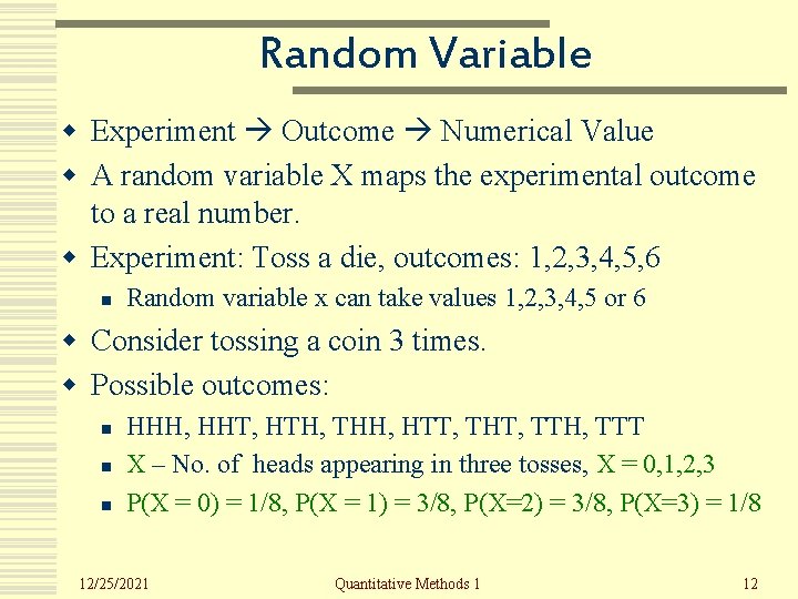
Random Variable w Experiment Outcome Numerical Value w A random variable X maps the experimental outcome to a real number. w Experiment: Toss a die, outcomes: 1, 2, 3, 4, 5, 6 n Random variable x can take values 1, 2, 3, 4, 5 or 6 w Consider tossing a coin 3 times. w Possible outcomes: n n n HHH, HHT, HTH, THH, HTT, THT, TTH, TTT X – No. of heads appearing in three tosses, X = 0, 1, 2, 3 P(X = 0) = 1/8, P(X = 1) = 3/8, P(X=2) = 3/8, P(X=3) = 1/8 12/25/2021 Quantitative Methods 1 12

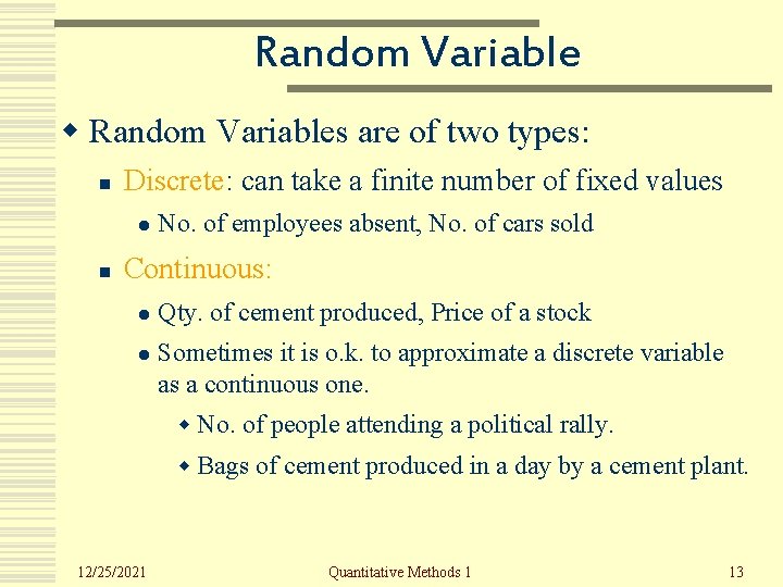
Random Variable w Random Variables are of two types: n Discrete: can take a finite number of fixed values l n No. of employees absent, No. of cars sold Continuous: l Qty. of cement produced, Price of a stock l Sometimes it is o. k. to approximate a discrete variable as a continuous one. w No. of people attending a political rally. w Bags of cement produced in a day by a cement plant. 12/25/2021 Quantitative Methods 1 13

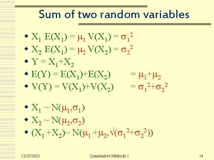
Sum of two random variables w X 1 E(X 1) = 1 V(X 1) = 12 w X 2 E(X 1) = 2 V(X 2) = 22 w Y = X 1+X 2 w E(Y) = E(X 1)+E(X 2) = 1+ 2 w V(Y) = V(X 1)+V(X 2) = 12+ 22 w X 1 ~ N( 1, 1) w X 2 ~ N( 2, 2) w (X 1 +X 2)~ N( 1 + 2, ( 12+ 22)) 12/25/2021 Quantitative Methods 1 14

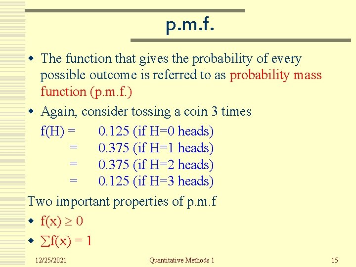
p. m. f. w The function that gives the probability of every possible outcome is referred to as probability mass function (p. m. f. ) w Again, consider tossing a coin 3 times f(H) = 0. 125 (if H=0 heads) = 0. 375 (if H=1 heads) = 0. 375 (if H=2 heads) = 0. 125 (if H=3 heads) Two important properties of p. m. f w f(x) 0 w f(x) = 1 12/25/2021 Quantitative Methods 1 15

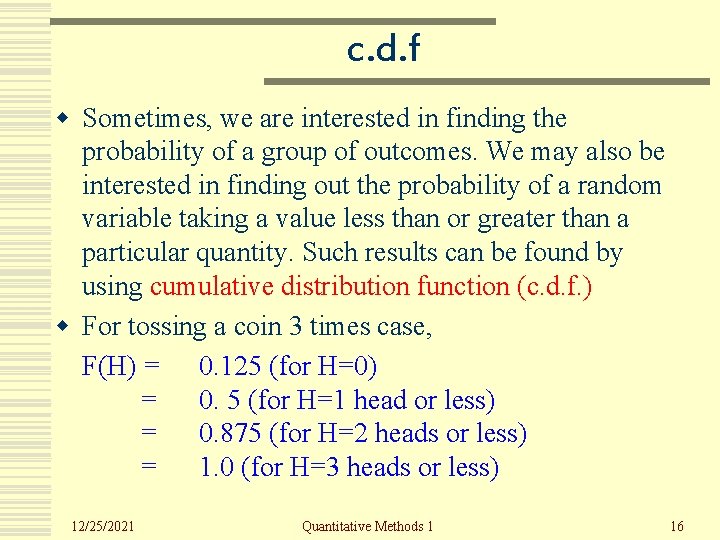
c. d. f w Sometimes, we are interested in finding the probability of a group of outcomes. We may also be interested in finding out the probability of a random variable taking a value less than or greater than a particular quantity. Such results can be found by using cumulative distribution function (c. d. f. ) w For tossing a coin 3 times case, F(H) = 0. 125 (for H=0) = 0. 5 (for H=1 head or less) = 0. 875 (for H=2 heads or less) = 1. 0 (for H=3 heads or less) 12/25/2021 Quantitative Methods 1 16

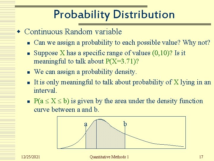
Probability Distribution w Continuous Random variable n n n Can we assign a probability to each possible value? Why not? Suppose X has a specific range of values (0, 10)? Is it meaningful to talk about P(X=3. 71)? We can assign a probability density. It is only meaningful to talk about probability of X lying in an interval. P(a X b) is given by the area under the density function curve between a and b. a 12/25/2021 b Quantitative Methods 1 17

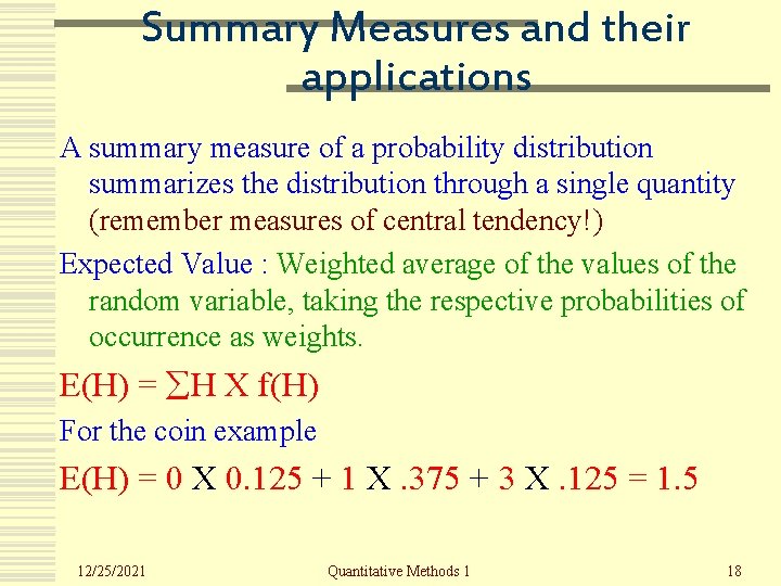
Summary Measures and their applications A summary measure of a probability distribution summarizes the distribution through a single quantity (remember measures of central tendency!) Expected Value : Weighted average of the values of the random variable, taking the respective probabilities of occurrence as weights. E(H) = H X f(H) For the coin example E(H) = 0 X 0. 125 + 1 X. 375 + 3 X. 125 = 1. 5 12/25/2021 Quantitative Methods 1 18

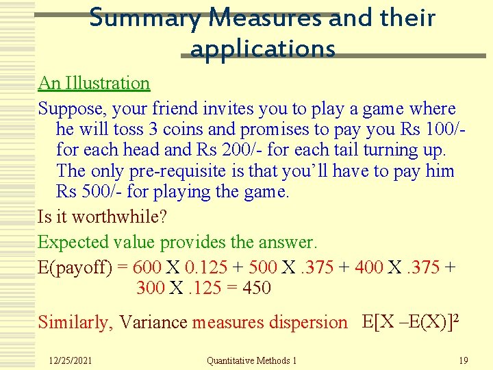
Summary Measures and their applications An Illustration Suppose, your friend invites you to play a game where he will toss 3 coins and promises to pay you Rs 100/for each head and Rs 200/- for each tail turning up. The only pre-requisite is that you’ll have to pay him Rs 500/- for playing the game. Is it worthwhile? Expected value provides the answer. E(payoff) = 600 X 0. 125 + 500 X. 375 + 400 X. 375 + 300 X. 125 = 450 Similarly, Variance measures dispersion E[X –E(X)]2 12/25/2021 Quantitative Methods 1 19

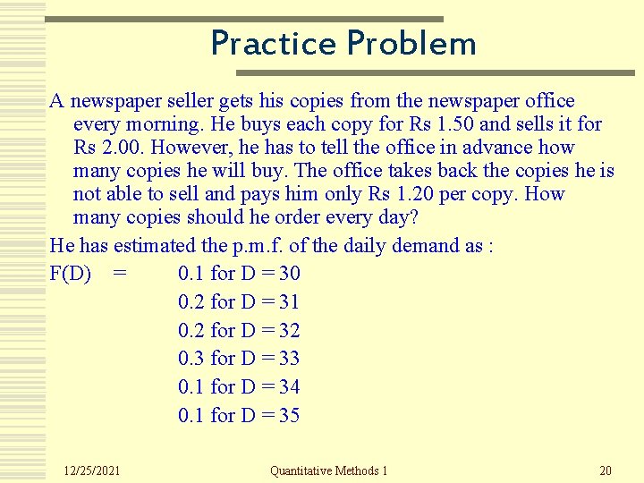
Practice Problem A newspaper seller gets his copies from the newspaper office every morning. He buys each copy for Rs 1. 50 and sells it for Rs 2. 00. However, he has to tell the office in advance how many copies he will buy. The office takes back the copies he is not able to sell and pays him only Rs 1. 20 per copy. How many copies should he order every day? He has estimated the p. m. f. of the daily demand as : F(D) = 0. 1 for D = 30 0. 2 for D = 31 0. 2 for D = 32 0. 3 for D = 33 0. 1 for D = 34 0. 1 for D = 35 12/25/2021 Quantitative Methods 1 20

12/25/2021 Quantitative Methods 1 21