Quantitative Genetics and Animal Breeding in the Age

Quantitative Genetics and Animal Breeding in the Age of Genomics Bruce Walsh

Classical Quantitative Genetics • Quantitative genetics deals with the observed variation in a trait both within and between populations • Basic model (Fisher 1918): The phenotype (z) is the sum of (unseen) genetic (g) and environmental values (e) • z=g+e • The genetic value needs to be further decomposed into an additive part A passed for parent to offspring, separate from dominance (D) and epistatic effects (I) that are only fully passed along in clones • g=A+D+I • Var(g)/Var(z) is quantitative measure of nature vs. nurture – fraction of all trait variation due to genetic differences

Fisher’s great insight: Phenotypic covariances between relatives can estimate the variances of g, e, etc. • For example, in the simplest settings, – Cov(parent, offspring) = Var(A)/2 – Cov(Full sibs) = Var(A)/2 + Var(D)/4 – Cov(clones) = Var(g) = Var(A)+Var(D)+Var(I) • Random-effects model • Thus, in classical quantitative genetics, a few statistical descriptors describe the underlying complex genetics – This leaves an uneasy feeling among most of my molecular colleagues. – Does the age of genomics usher in the death knell of Quantitative Genetics?

“Classical” Animal Breeding • Using the records (phenotypes) of individuals from a known (often very complex) pedigree, estimates for the breeding values (A) for individuals are obtained – This is usually done using the machinery of BLUP -- best linear unbiased predictor. – To do this, we also have to estimate Var(A), typically this is done using REML -- restricted (or residual) maximum likelihood • Predicted value of offspring from two parents is the average of the parental breeding values • How will genomics alter this classical approach?

Approximate costs of genome projects • Arabidopsis Genome Project. . . $500 million • Drosophila Genome Project. . . $1 billion • Human Genome Project. . . $10 billion • Working knowledge of multivariate statistics. . . Priceless

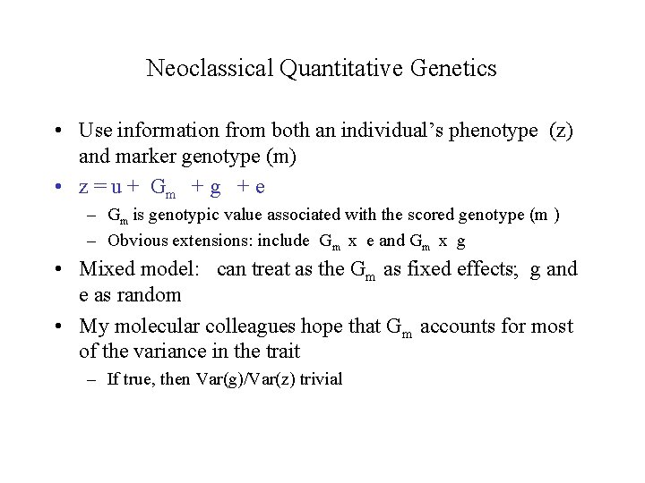
Neoclassical Quantitative Genetics • Use information from both an individual’s phenotype (z) and marker genotype (m) • z = u + Gm + g + e – Gm is genotypic value associated with the scored genotype (m ) – Obvious extensions: include Gm x e and Gm x g • Mixed model: can treat as the Gm as fixed effects; g and e as random • My molecular colleagues hope that Gm accounts for most of the variance in the trait – If true, then Var(g)/Var(z) trivial

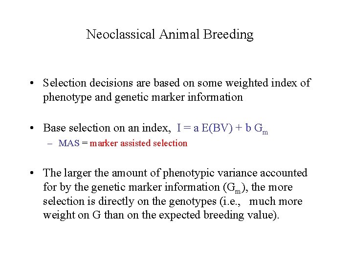
Neoclassical Animal Breeding • Selection decisions are based on some weighted index of phenotype and genetic marker information • Base selection on an index, I = a E(BV) + b Gm – MAS = marker assisted selection • The larger the amount of phenotypic variance accounted for by the genetic marker information (Gm), the more selection is directly on the genotypes (i. e. , much more weight on G than on the expected breeding value).

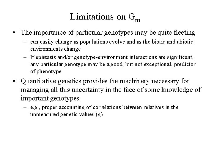
Limitations on Gm • The importance of particular genotypes may be quite fleeting – can easily change as populations evolve and as the biotic and abiotic environments change – If epistasis and/or genotype-environment interactions are significant, any particular genotype may be a good, but not exceptional, predictor of phenotype • Quantitative genetics provides the machinery necessary for managing all this uncertainty in the face of some knowledge of important genotypes – e. g. , proper accounting of correlations between relatives in the unmeasured genetic values (g)

Limitations with MAS • Tradeoff between increased short-term response under MAS vs. decreased short-term response compared with phenotypic selection. – Reduced selection on phenotype – Reduction in effective population size • MAS may not be cost-effective compared to phenotypic selection • Optimal setting for MAS – Genes of major effect (e. g. , scrapie (prion) resistance) – Sex-limited expression – Traits difficult/expensive to score directly (i. e. , carcass traits)

How do we obtain Gm? • Ideally, we screen a number of candidate loci • QTL (Quantitative trait locus) mapping • Uses molecular markers to follow which chromosome segments are common between individuals • This allows construction of a likelihood function, e. g. ,

A typical QTL map from a likelihood analysis

Genomics and candidate loci • Typical QTL confidence interval 20 -50 c. M • The big question: how do we find suitable candidates? • The hope is that a genomic sequence will suggest candidates

Genomics tools to probe for candidates • Dense marker maps • Complete genome sequence – Expression data (microarrays) – Proteomics – Metablomics

The accelerating pace of genomics • Faster and cheaper sequencing • Rapid screening of thousands of loci via DNA chips • Phylogenetic bootstrapping from model systems to distant relatives

Prediction of Candidate Genes • Try homologous candidates from other species • Examine all Open Reading Frames (ORFs) within a QTL confidence interval – Expression array analysis of these ORFs – Lack of tissue-specific expression does not exclude a gene • Proteomics – Specific protein motifs may provide functional clues • Cracking the regulatory code (in silico genetics)

Searching for Natural Variation • This may be the area where genomics has the largest payoff • Source (natural and/or weakly domesticated) populations contain more variation than the current highly domesticated lines • Key is to first detect and localize importance variants, then introgress them into elite lines

The impact of other biotechnologies • Cloning, other reproductive technologies – – Maintain elite lines as cell cultures? Trans-species maintenance of tissue cultures Embryo transplantation into elite maternal lines? Creation of permanently heterotic lines • Transgenics – Important tool in both breeding and evolutionary biology • Complications: – Silencing of multiple copies in some species – Strong position effects – Currently restricted to major genes • Major genes can have deleterious effects on other characters • Importance of quantitative genetics for selecting for background polygenic modifiers

Useful Tools for Quantitative Genetic analysis • Four subfields of Quantitative Genetics – – Plant breeding Animal breeding (forest genetics) Evolutionary Genetics Human Genetics • Restricted communications between fields • Important tools often unknown outside a field

Tools from Plant Breeding • Special features dealt with by plant breeders – Diversity of mating systems (esp. selfing) – Sessile individuals • Issues – – Creation and selection of inbred lines Hybridization between lines Genotype x Environment interactions Competition • Plant breeding tools useful in Animal Breeding – Field-plot designs – G x E analysis models: AMMI and biplots • These designs are also excellent candidates for the analysis of microarray expression data – Covariance between inbred relatives – Line cross analysis

Animal Breeding • Special features – – Complex pedigrees Large half-sib (more rarely full-sib) families Long life spans Overlapping generations • Tree breeders face many of these same issues • Animal breeding tools useful in other fields – BLUP (best linear unbiased predictors) for genotypic values – REML (restricted maximum likelihood) for variance components • BLUP/REML allow for arbitrary pedigrees, very complex models – Maternal effects designs • Endosperm work of Shaw and Waser – Selection response in structured populations

Evolutionary Genetics • Issues – Estimating the nature and amount of selection – Population-genetic models of evolution • Tools – Estimation of the nature of natural selection on any specified character • Lande-Arnold fitness estimation; cubic splines – Using DNA sequences to detect selection on a locus • Example: teosinte-branched 1 – Coalescent theory • The genealogy of DNA sequences within a random sample – Analysis of finite-locus and non-Gaussian models of selection response • Barton and Turelli; Burger

Human Genetics • Issues – Very small family sizes – Lack of controlled mating designs • Tools of potential use – Sib-pair approaches for QTL mapping • QTL mapping in populations – Transmission-disequilibrium test (TDT) • Account for population structure – Linkage-disequilibrium mapping • Use historical recombinations to fine-map genes – Random-effects models for QTL mapping • BLUP/REML-type analysis over arbitrary pedigrees

Conclusions • Genomics will increase, not decrease, the importance of quantitative genetics • The machinery of classical quantitative genetics is easily modified to account for massive advances in genomics and other fields of biotechonology • Useful and powerful tools have been developed to address specific issues in the various subfields of quantitative genetics • The future of animal breeding is a natural fusion of genomic information into an expanded quantitativegenetics framework, exploiting advances in reproductive biotechnologies.