Quantifying Uncertainty in Inverse Problems Workshop on Statistical

Quantifying Uncertainty in Inverse Problems Workshop on Statistical Methods for Inverse Problems Institute for Pure and Applied Mathematics University of California, Los Angeles 5 -6 November 2003 P. B. Stark Department of Statistics University of California Berkeley, CA 94720 -3860 www. stat. berkeley. edu/~stark

Abstract Some qualitative and quantitative statistical measures of uncertainty apply to inverse problems. Decision theory provides a framework for thinking about inverse problems. The intrinsic uncertainty in an inverse problem usually is not equal to the uncertainty of a “solution” to the inverse problem constructed by any particular technique. The intrinsic uncertainty depends crucially on the prior constraints on the unknown (including prior probability distributions in the case of Bayesian analyses), on the forward operator, on the distribution of the observational errors, and on the kinds of properties of the unknown one wishes to estimate. Some aspects of uncertainty in inverse problems can be understood geometrically.

My Assumptions about You • All of you know much more math than I do. • I know a little more statistics than some of you do. • You haven’t heard me talk about this before. • You are more interested in theory than numerical algorithms or specific applications.

Outline • Inverse Problems as Statistics – Ingredients; Models – Forward and Inverse Problems—applied perspective – Statistical point of view – Some connections • Notation; linear problems; illustration – Example: geomagnetism from satellite observations • Qualitative uncertainty: Identifiability and uniqueness – Sketch of identifiablity and extremal modeling – Backus-Gilbert theory & extensions

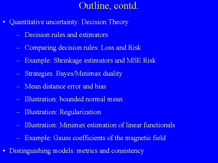
Outline, contd. • Quantitative uncertainty: Decision Theory – Decision rules and estimators – Comparing decision rules: Loss and Risk – Example: Shrinkage estimators and MSE Risk – Strategies. Bayes/Minimax duality – Mean distance error and bias – Illustration: bounded normal mean – Illustration: Regularization – Illustration: Minimax estimation of linear functionals – Example: Gauss coefficients of the magnetic field • Distinguishing models: metrics and consistency

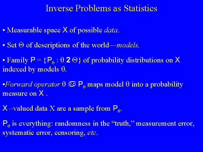
Inverse Problems as Statistics • Measurable space X of possible data. • Set of descriptions of the world—models. • Family P = {P : 2 } of probability distributions on X indexed by models . • Forward operator P maps model into a probability measure on X. X –valued data X are a sample from P. P is everything: randomness in the “truth, ” measurement error, systematic error, censoring, etc.

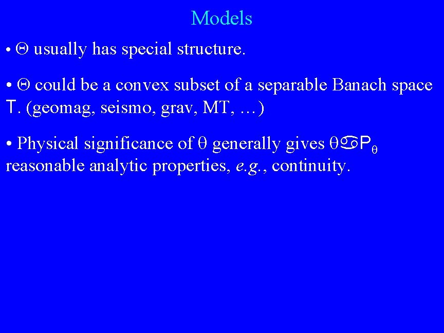
Models • usually has special structure. • could be a convex subset of a separable Banach space T. (geomag, seismo, grav, MT, …) • Physical significance of generally gives P reasonable analytic properties, e. g. , continuity.

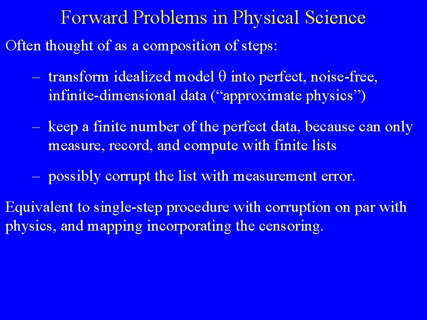
Forward Problems in Physical Science Often thought of as a composition of steps: – transform idealized model into perfect, noise-free, infinite-dimensional data (“approximate physics”) – keep a finite number of the perfect data, because can only measure, record, and compute with finite lists – possibly corrupt the list with measurement error. Equivalent to single-step procedure with corruption on par with physics, and mapping incorporating the censoring.

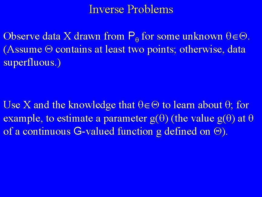
Inverse Problems Observe data X drawn from Pθ for some unknown . (Assume contains at least two points; otherwise, data superfluous. ) Use X and the knowledge that to learn about ; for example, to estimate a parameter g( ) (the value g(θ) at θ of a continuous G-valued function g defined on ).

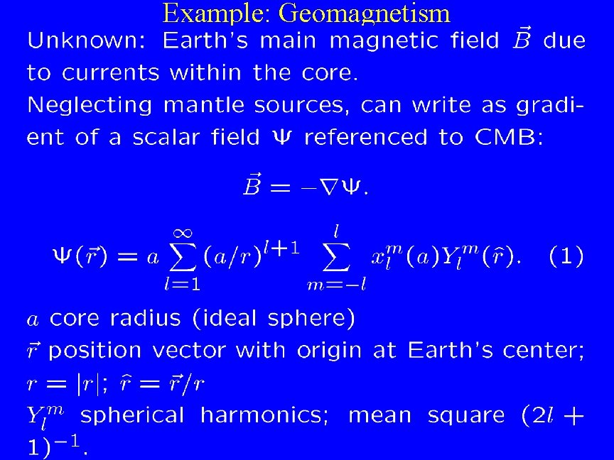
Example: Geomagnetism

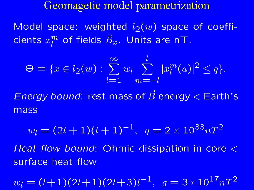
Geomagetic model parametrization

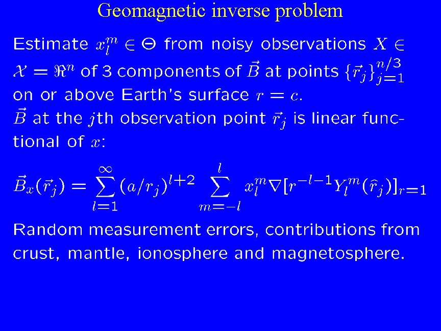
Geomagnetic inverse problem

Inverse Problems in Physical Science Inverse problems in science often “solved” using applied math methods for Ill-posed problems (e. g. , Tichonov regularization, analytic inversions) Those methods are designed to answer different questions; can behave poorly with data (e. g. , bad bias & variance) Inference construction: Statistical viewpoint may be more appropriate for interpreting real data with stochastic errors.

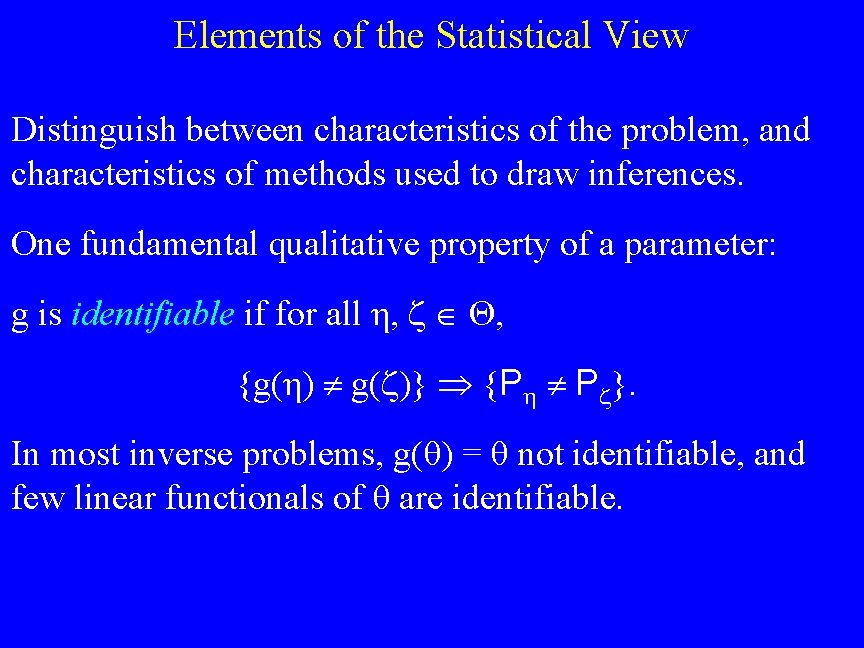
Elements of the Statistical View Distinguish between characteristics of the problem, and characteristics of methods used to draw inferences. One fundamental qualitative property of a parameter: g is identifiable if for all η, Θ, {g(η) g( )} {P P }. In most inverse problems, g(θ) = θ not identifiable, and few linear functionals of θ are identifiable.

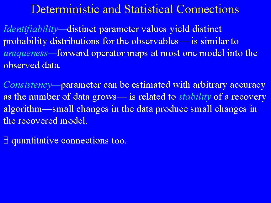
Deterministic and Statistical Connections Identifiability—distinct parameter values yield distinct probability distributions for the observables— is similar to uniqueness—forward operator maps at most one model into the observed data. Consistency—parameter can be estimated with arbitrary accuracy as the number of data grows— is related to stability of a recovery algorithm—small changes in the data produce small changes in the recovered model. quantitative connections too.

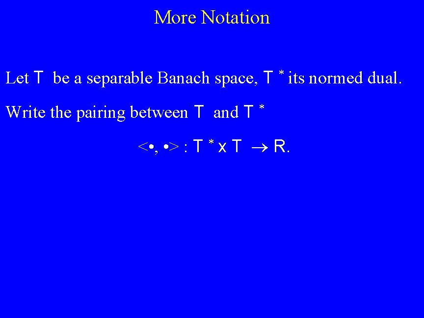
More Notation Let T be a separable Banach space, T * its normed dual. Write the pairing between T and T * < • , • > : T * x T R.

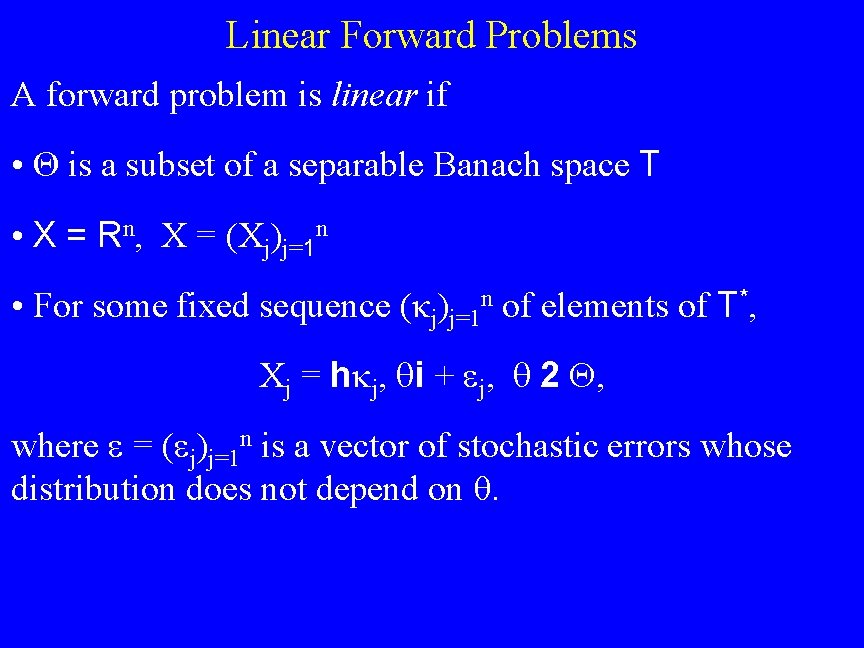
Linear Forward Problems A forward problem is linear if • Θ is a subset of a separable Banach space T • X = Rn, X = (Xj)j=1 n • For some fixed sequence (κj)j=1 n of elements of T*, Xj = h j, i + j, 2 , where = ( j)j=1 n is a vector of stochastic errors whose distribution does not depend on θ.

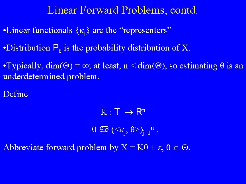
Linear Forward Problems, contd. • Linear functionals {κj} are the “representers” • Distribution Pθ is the probability distribution of X. • Typically, dim(Θ) = ; at least, n < dim(Θ), so estimating θ is an underdetermined problem. Define K : T Rn (<κj, θ>)j=1 n. Abbreviate forward problem by X = Kθ + ε, θ Θ.

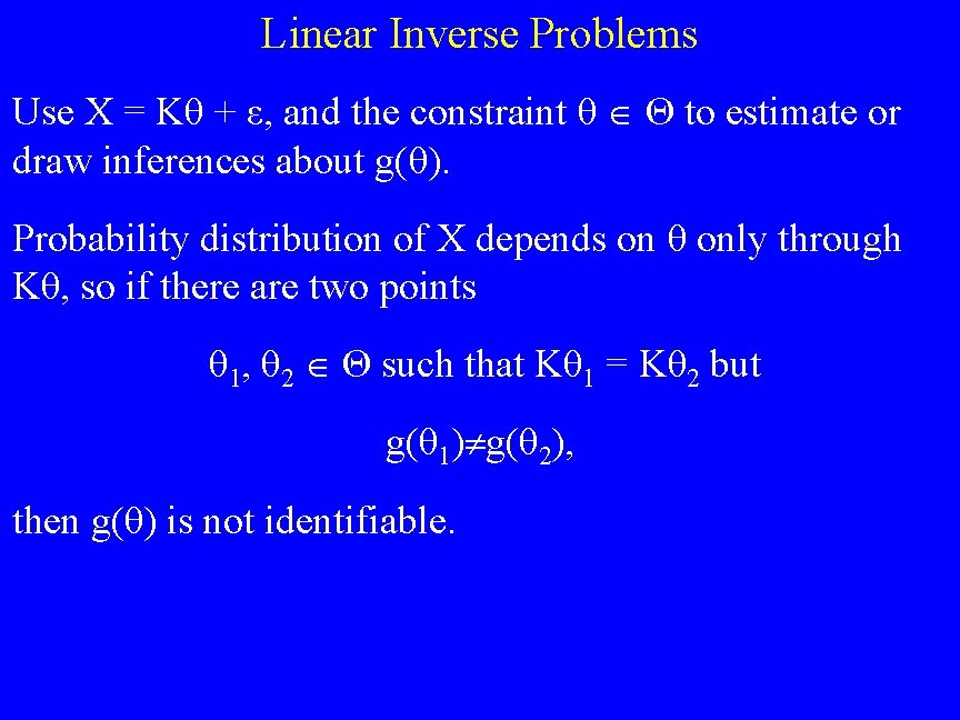
Linear Inverse Problems Use X = Kθ + ε, and the constraint θ Θ to estimate or draw inferences about g(θ). Probability distribution of X depends on θ only through Kθ, so if there are two points θ 1, θ 2 Θ such that Kθ 1 = Kθ 2 but g(θ 1) g(θ 2), then g(θ) is not identifiable.

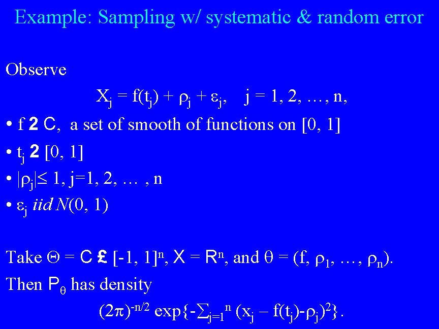
Example: Sampling w/ systematic & random error Observe Xj = f(tj) + j, j = 1, 2, …, n, • f 2 C, a set of smooth of functions on [0, 1] • tj 2 [0, 1] • | j| 1, j=1, 2, … , n • j iid N(0, 1) Take = C £ [-1, 1]n, X = Rn, and = (f, 1, …, n). Then P has density (2 )-n/2 exp{- j=1 n (xj – f(tj)- j)2}.

Sketch: Identifiability {P = P } ; { = }, so not identifiable g cannot be estimated with bounded bias {P = P } ; {g( ) = g( )}, so g not identifiable

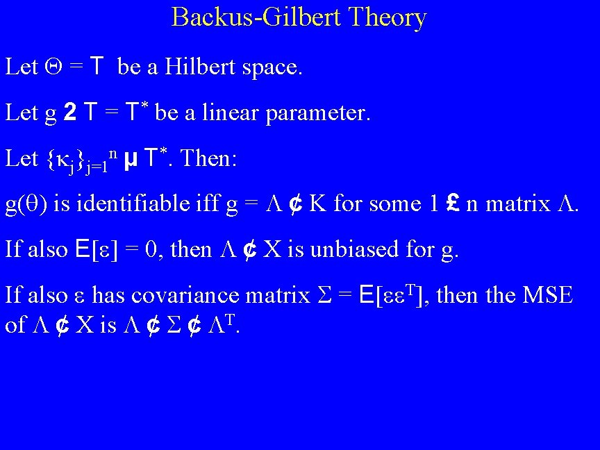
Backus-Gilbert Theory Let = T be a Hilbert space. Let g 2 T = T* be a linear parameter. Let { j}j=1 n µ T*. Then: g( ) is identifiable iff g = ¢ K for some 1 £ n matrix . If also E[ ] = 0, then ¢ X is unbiased for g. If also has covariance matrix = E[ T], then the MSE of ¢ X is ¢ ¢ T.

Sketch: Backus-Gilbert

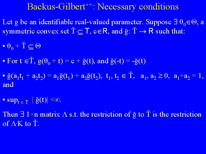
Backus-Gilbert++: Necessary conditions Let g be an identifiable real-valued parameter. Suppose θ 0 Θ, a symmetric convex set Ť T, c R, and ğ: Ť R such that: • θ 0 + Ť Θ • For t Ť, g(θ 0 + t) = c + ğ(t), and ğ(-t) = -ğ(t) • ğ(a 1 t 1 + a 2 t 2) = a 1ğ(t 1) + a 2ğ(t 2), t 1, t 2 Ť, a 1, a 2 0, a 1+a 2 = 1, and • supt Ť | ğ(t)| <. Then 1×n matrix Λ s. t. the restriction of ğ to Ť is the restriction of Λ. K to Ť.

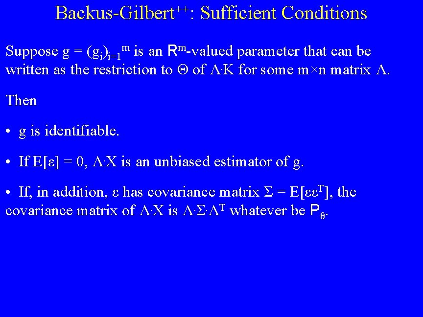
Backus-Gilbert++: Sufficient Conditions Suppose g = (gi)i=1 m is an Rm-valued parameter that can be written as the restriction to Θ of Λ. K for some m×n matrix Λ. Then • g is identifiable. • If E[ε] = 0, Λ. X is an unbiased estimator of g. • If, in addition, ε has covariance matrix Σ = E[εεT], the covariance matrix of Λ. X is Λ. Σ. ΛT whatever be Pθ.

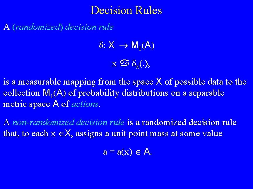
Decision Rules A (randomized) decision rule δ: X M 1(A) x δx(. ), is a measurable mapping from the space X of possible data to the collection M 1(A) of probability distributions on a separable metric space A of actions. A non-randomized decision rule is a randomized decision rule that, to each x X, assigns a unit point mass at some value a = a(x) A.

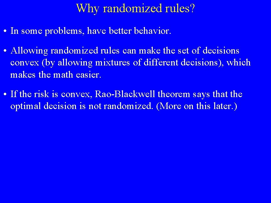
Why randomized rules? • In some problems, have better behavior. • Allowing randomized rules can make the set of decisions convex (by allowing mixtures of different decisions), which makes the math easier. • If the risk is convex, Rao-Blackwell theorem says that the optimal decision is not randomized. (More on this later. )

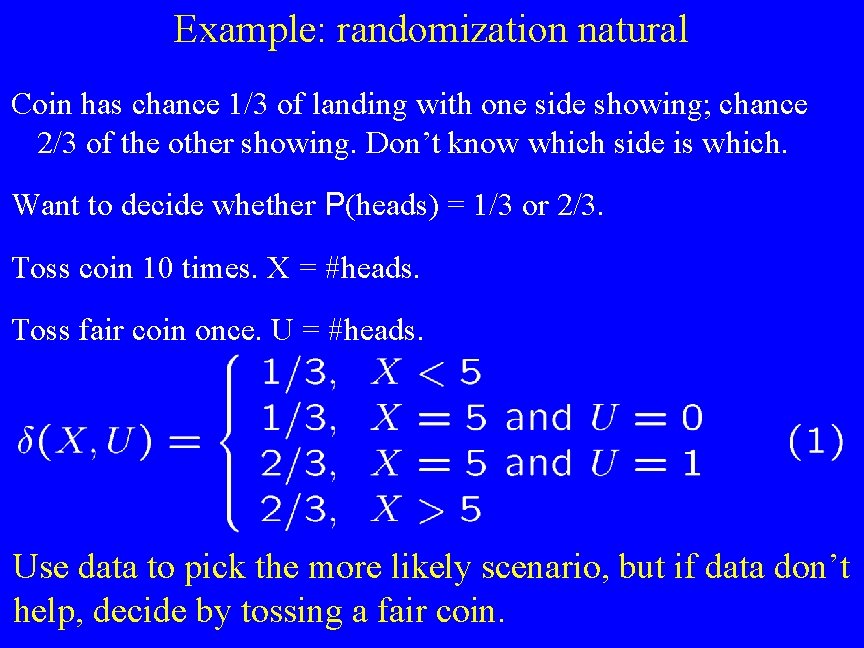
Example: randomization natural Coin has chance 1/3 of landing with one side showing; chance 2/3 of the other showing. Don’t know which side is which. Want to decide whether P(heads) = 1/3 or 2/3. Toss coin 10 times. X = #heads. Toss fair coin once. U = #heads. Use data to pick the more likely scenario, but if data don’t help, decide by tossing a fair coin.

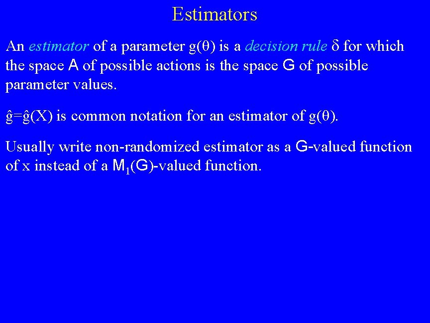
Estimators An estimator of a parameter g(θ) is a decision rule for which the space A of possible actions is the space G of possible parameter values. ĝ=ĝ(X) is common notation for an estimator of g(θ). Usually write non-randomized estimator as a G-valued function of x instead of a M 1(G)-valued function.

Comparing Decision Rules Infinitely many decision rules and estimators. Which one to use? The best one! But what does best mean?

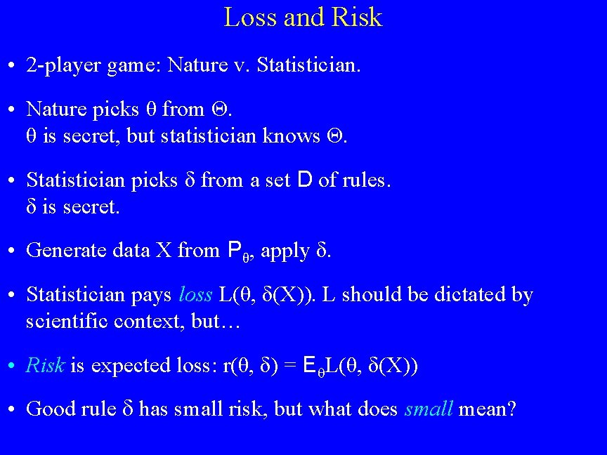
Loss and Risk • 2 -player game: Nature v. Statistician. • Nature picks θ from Θ. θ is secret, but statistician knows Θ. • Statistician picks δ from a set D of rules. δ is secret. • Generate data X from Pθ, apply δ. • Statistician pays loss L(θ, δ(X)). L should be dictated by scientific context, but… • Risk is expected loss: r(θ, δ) = E L(θ, δ(X)) • Good rule has small risk, but what does small mean?

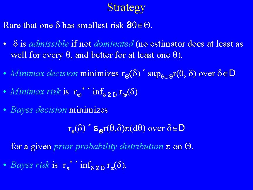
Strategy Rare that one has smallest risk 8 • is admissible if not dominated (no estimator does at least as well for every , and better for at least one . • Minimax decision minimizes r ( ) ´ sup r(θ, δ) over D • Minimax risk is r * ´ inf 2 D r (δ) • Bayes decision minimizes r ( ) ´ s r( , ) (d ) over D for a given prior probability distribution on • Bayes risk is r * ´ inf 2 D r ( ).

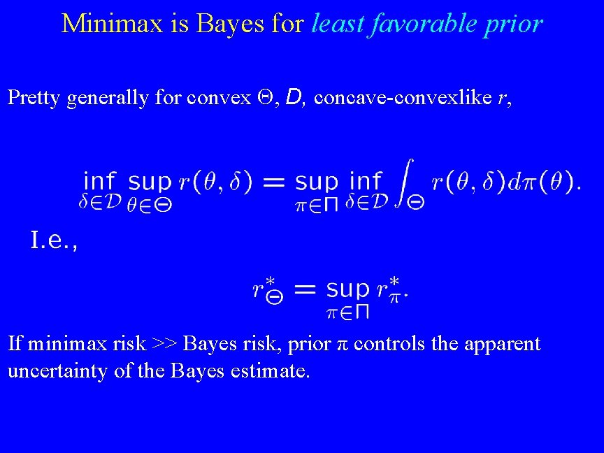
Minimax is Bayes for least favorable prior Pretty generally for convex D, concave-convexlike r, If minimax risk >> Bayes risk, prior π controls the apparent uncertainty of the Bayes estimate.

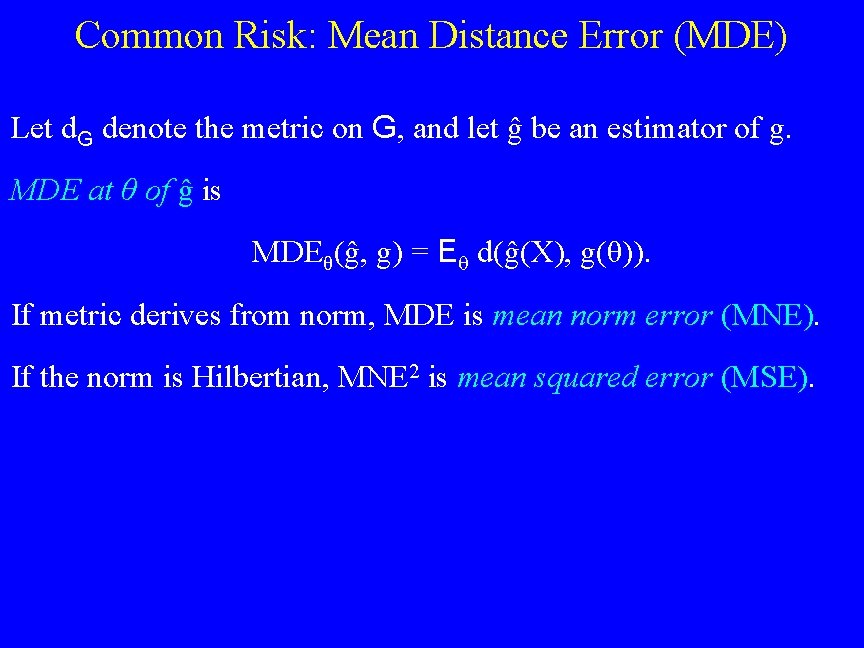
Common Risk: Mean Distance Error (MDE) Let d. G denote the metric on G, and let ĝ be an estimator of g. MDE at θ of ĝ is MDEθ(ĝ, g) = E d(ĝ(X), g(θ)). If metric derives from norm, MDE is mean norm error (MNE). If the norm is Hilbertian, MNE 2 is mean squared error (MSE).

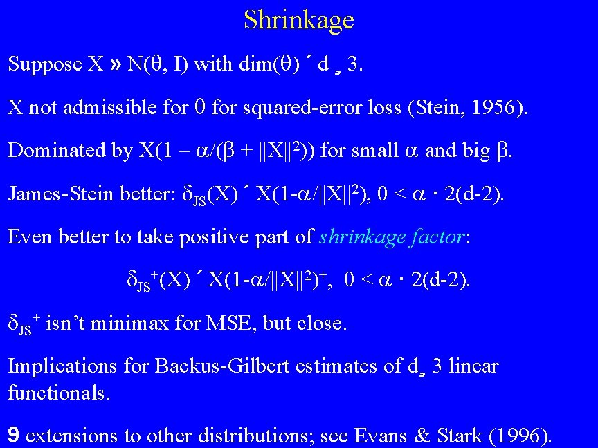
Shrinkage Suppose X » N( , I) with dim( ) ´ d ¸ 3. X not admissible for squared-error loss (Stein, 1956). Dominated by X(1 – /( + ||X||2)) for small and big . James-Stein better: JS(X) ´ X(1 - /||X||2), 0 < · 2(d-2). Even better to take positive part of shrinkage factor: JS+(X) ´ X(1 - /||X||2)+, 0 < · 2(d-2). JS+ isn’t minimax for MSE, but close. Implications for Backus-Gilbert estimates of d¸ 3 linear functionals. 9 extensions to other distributions; see Evans & Stark (1996).

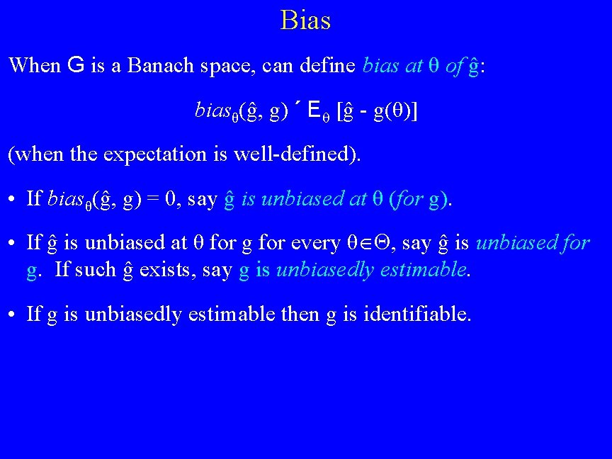
Bias When G is a Banach space, can define bias at θ of ĝ: biasθ(ĝ, g) ´ E [ĝ - g(θ)] (when the expectation is well-defined). • If biasθ(ĝ, g) = 0, say ĝ is unbiased at θ (for g). • If ĝ is unbiased at θ for g for every θ , say ĝ is unbiased for g. If such ĝ exists, say g is unbiasedly estimable. • If g is unbiasedly estimable then g is identifiable.

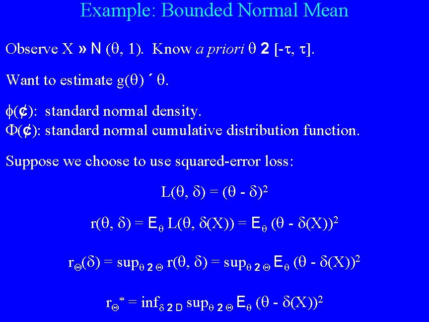
Example: Bounded Normal Mean Observe X » N ( , ). Know a priori 2 [- , ]. Want to estimate g( ´ (¢): standard normal density. (¢): standard normal cumulative distribution function. Suppose we choose to use squared-error loss: L( , ) = ( - )2 r( , ) = E L( , (X)) = E ( - (X))2 r ( ) = sup 2 r( , ) = sup 2 E ( - (X))2 r = inf 2 D sup 2 E ( - (X))2

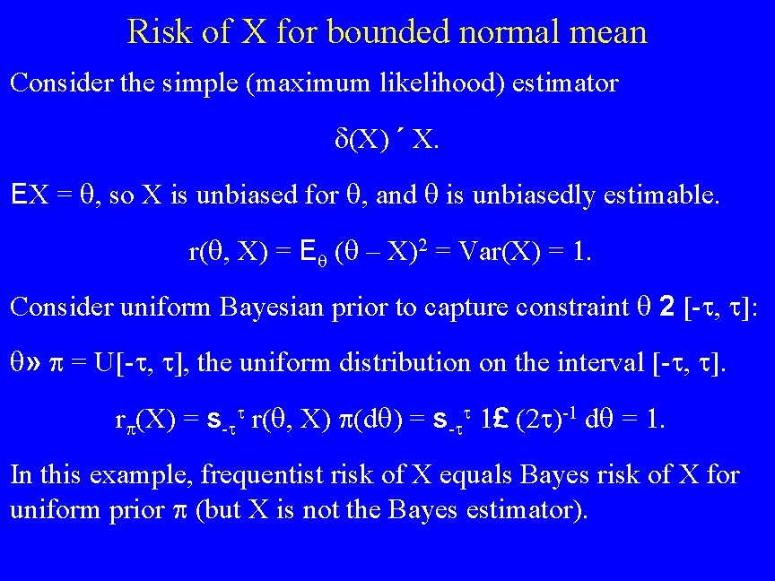
Risk of X for bounded normal mean Consider the simple (maximum likelihood) estimator (X) ´ X. EX = , so X is unbiased for , and is unbiasedly estimable. r( , X) = E ( – X)2 = Var(X) = . Consider uniform Bayesian prior to capture constraint 2 [- , ]: » = U[- , ], the uniform distribution on the interval [- , ]. r (X) = s- r( , X) (d ) = s- £ (2 )-1 d = . In this example, frequentist risk of X equals Bayes risk of X for uniform prior (but X is not the Bayes estimator).

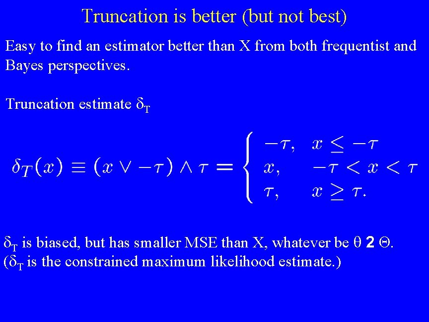
Truncation is better (but not best) Easy to find an estimator better than X from both frequentist and Bayes perspectives. Truncation estimate T T is biased, but has smaller MSE than X, whatever be 2 is the constrained maximum likelihood estimate. )

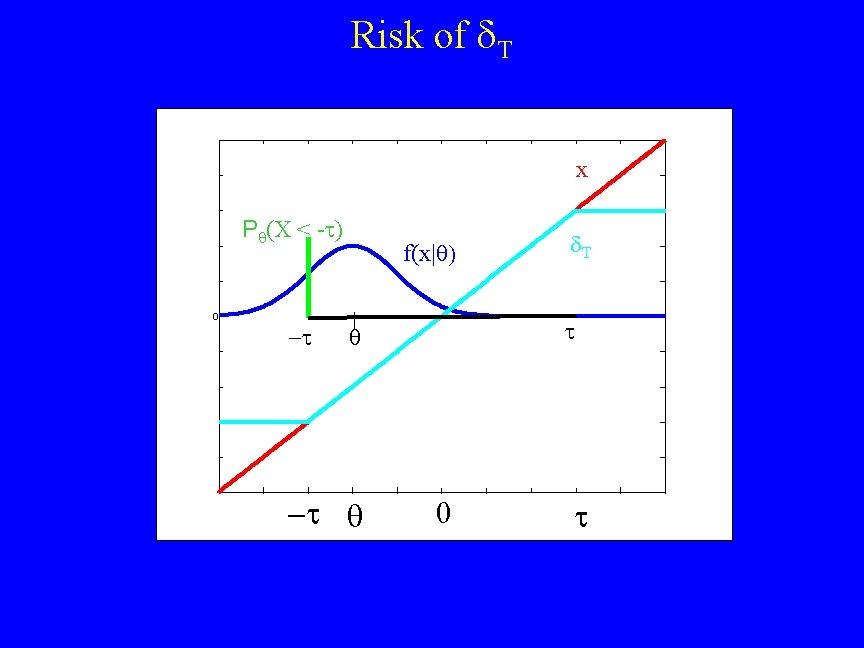
Risk of T x P (X < - ) 0 f(x| T 0

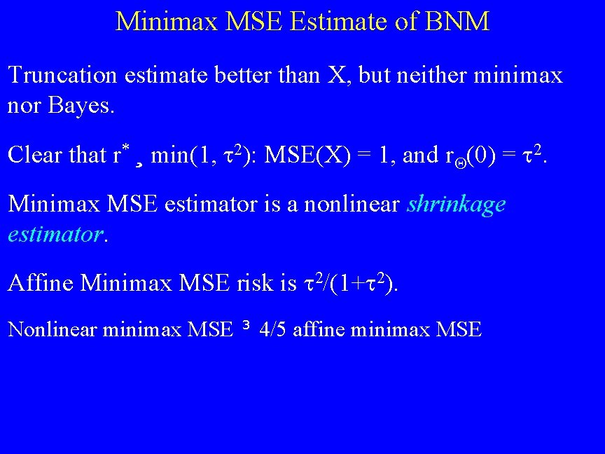
Minimax MSE Estimate of BNM Truncation estimate better than X, but neither minimax nor Bayes. Clear that r* ¸ min(1, 2): MSE(X) = 1, and r (0) = 2. Minimax MSE estimator is a nonlinear shrinkage estimator. Affine Minimax MSE risk is 2/(1+ 2). Nonlinear minimax MSE ³ 4/5 affine minimax MSE

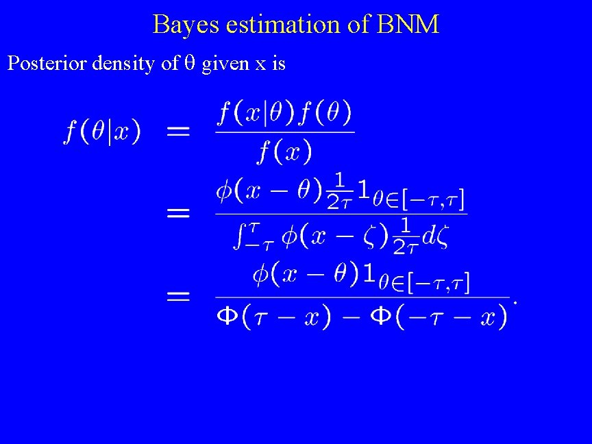
Bayes estimation of BNM Posterior density of given x is

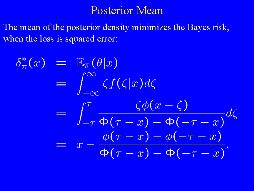
Posterior Mean The mean of the posterior density minimizes the Bayes risk, when the loss is squared error:

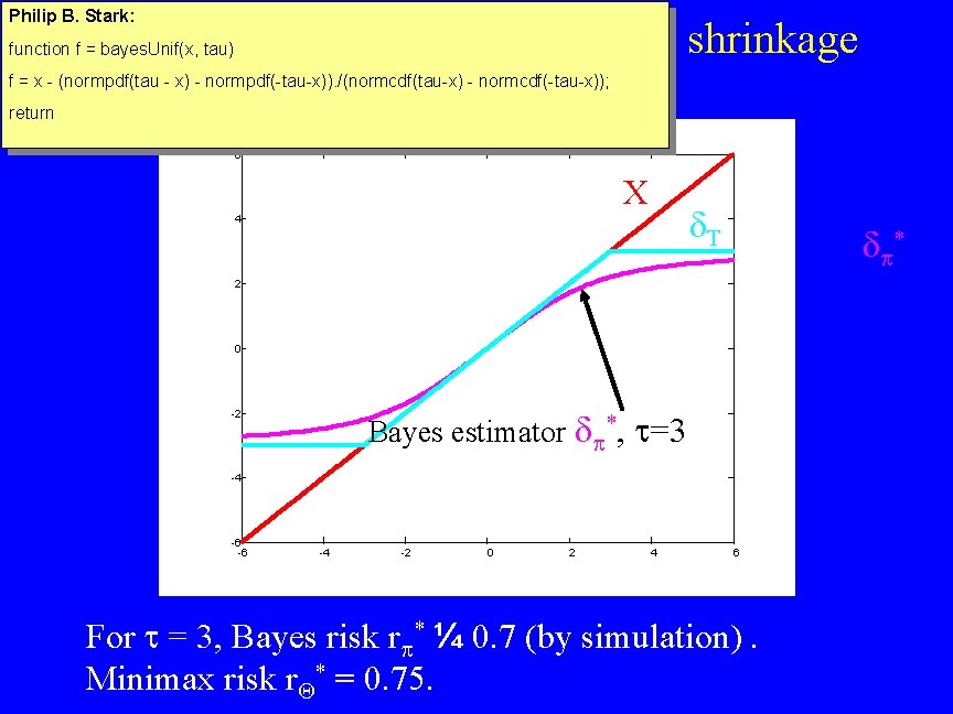
Philip B. Stark: Bayes estimator is also nonlinear shrinkage function f = bayes. Unif(x, tau) f = x - (normpdf(tau - x) - normpdf(-tau-x)). /(normcdf(tau-x) - normcdf(-tau-x)); return 6 X T 4 * 2 0 Bayes estimator *, =3 -2 -4 -6 -6 -4 -2 0 2 4 6 For = 3, Bayes risk r * ¼ 0. 7 (by simulation). Minimax risk r * = 0. 75.

Bayes/Minimax Risks Difference between knowing 2 [- , ], and » U[- , ].

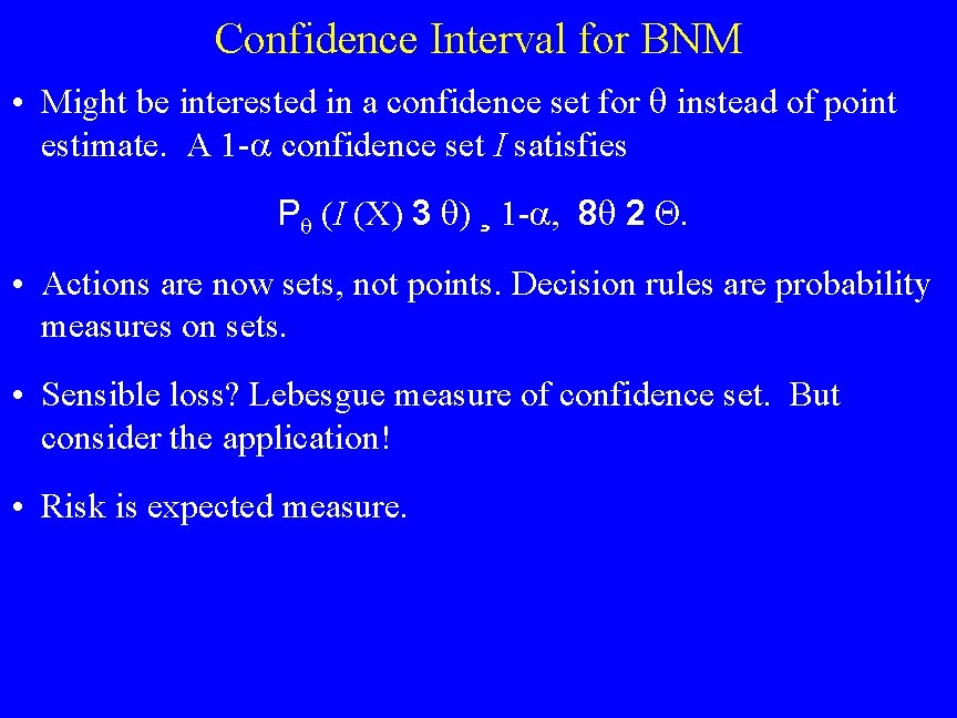
Confidence Interval for BNM • Might be interested in a confidence set for instead of point estimate. A 1 - confidence set I satisfies P (I (X) 3 ) ¸ 1 - , 8 2 • Actions are now sets, not points. Decision rules are probability measures on sets. • Sensible loss? Lebesgue measure of confidence set. But consider the application! • Risk is expected measure.

Some Confidence Procedures • Naïve: • Truncated: [X – z /2, X+ z /2] Å [- , ] • Affine fixed-length: [a. X+b– /2, a. X+b+ /2] • Nonlinear fixed length: [f(X)– /2, f(X)+ /2], f measurable • Variable length: [l(X), u(X)], l, u measurable • Likelihood ratio test (LRT): Include all 2 [- , ] s. t. ( )/ (0) ¸ c. Choose c to get 1 - coverage.

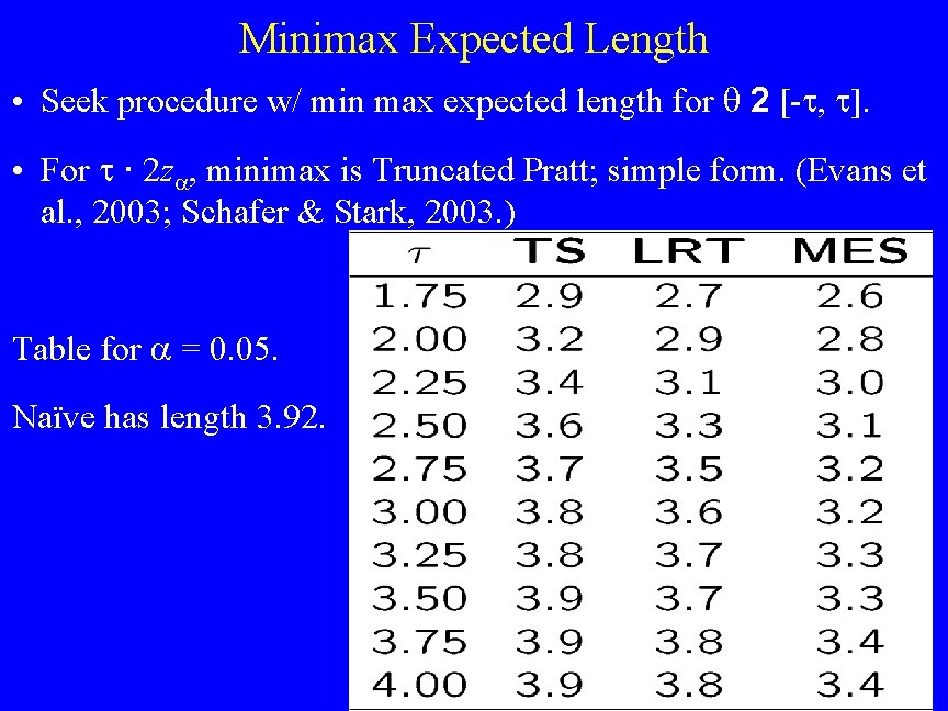
Minimax Expected Length • Seek procedure w/ min max expected length for 2 [- , ]. • For · 2 z , minimax is Truncated Pratt; simple form. (Evans et al. , 2003; Schafer & Stark, 2003. ) Table for = 0. 05. Naïve has length 3. 92.

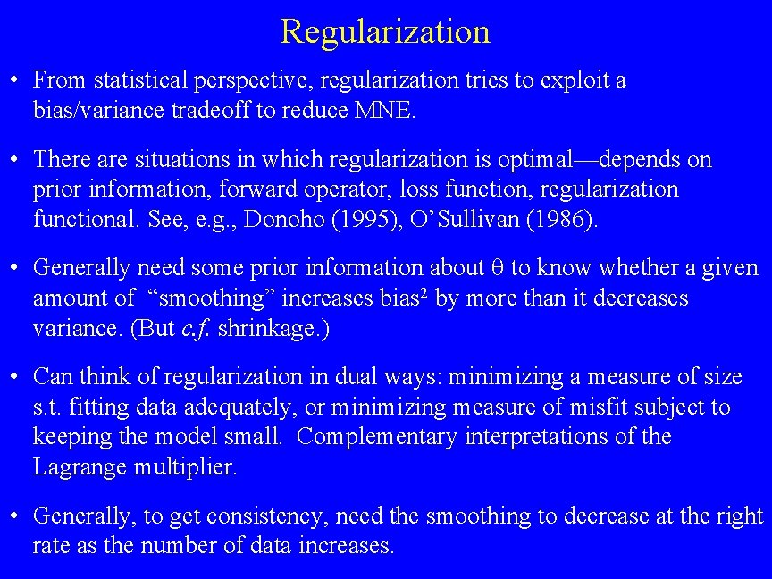
Regularization • From statistical perspective, regularization tries to exploit a bias/variance tradeoff to reduce MNE. • There are situations in which regularization is optimal—depends on prior information, forward operator, loss function, regularization functional. See, e. g. , Donoho (1995), O’Sullivan (1986). • Generally need some prior information about to know whether a given amount of “smoothing” increases bias 2 by more than it decreases variance. (But c. f. shrinkage. ) • Can think of regularization in dual ways: minimizing a measure of size s. t. fitting data adequately, or minimizing measure of misfit subject to keeping the model small. Complementary interpretations of the Lagrange multiplier. • Generally, to get consistency, need the smoothing to decrease at the right rate as the number of data increases.

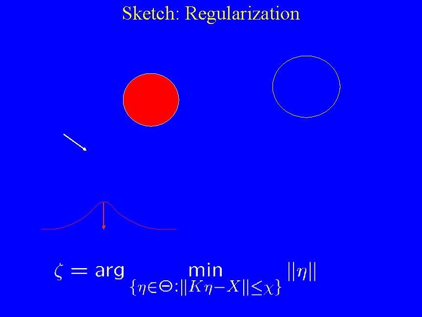
Sketch: Regularization

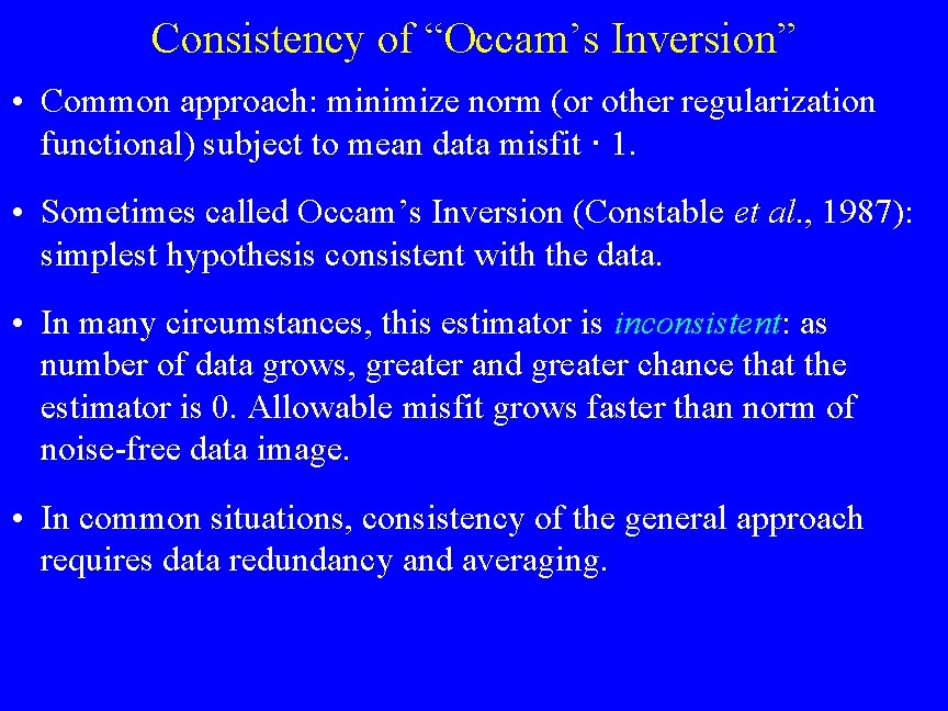
Consistency of “Occam’s Inversion” • Common approach: minimize norm (or other regularization functional) subject to mean data misfit · 1. • Sometimes called Occam’s Inversion (Constable et al. , 1987): simplest hypothesis consistent with the data. • In many circumstances, this estimator is inconsistent: as number of data grows, greater and greater chance that the estimator is 0. Allowable misfit grows faster than norm of noise-free data image. • In common situations, consistency of the general approach requires data redundancy and averaging.

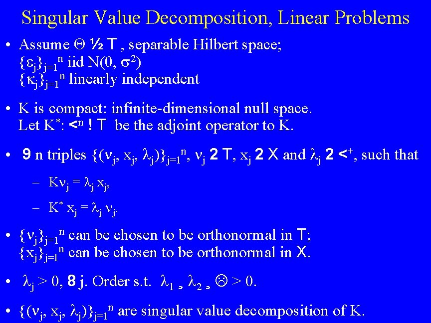
Singular Value Decomposition, Linear Problems • Assume ½ T , separable Hilbert space; { j}j=1 n iid N(0, 2) { j}j=1 n linearly independent • K is compact: infinite-dimensional null space. Let K*: <n ! T be the adjoint operator to K. • 9 n triples {( j, xj, j)}j=1 n, j 2 T, xj 2 X and j 2 <+, such that – K j = j xj, – K* xj = j j. • { j}j=1 n can be chosen to be orthonormal in T; {xj}j=1 n can be chosen to be orthonormal in X. • j > 0, 8 j. Order s. t. 1 ¸ 2 ¸ > 0. • {( j, xj, j)}j=1 n are singular value decomposition of K.

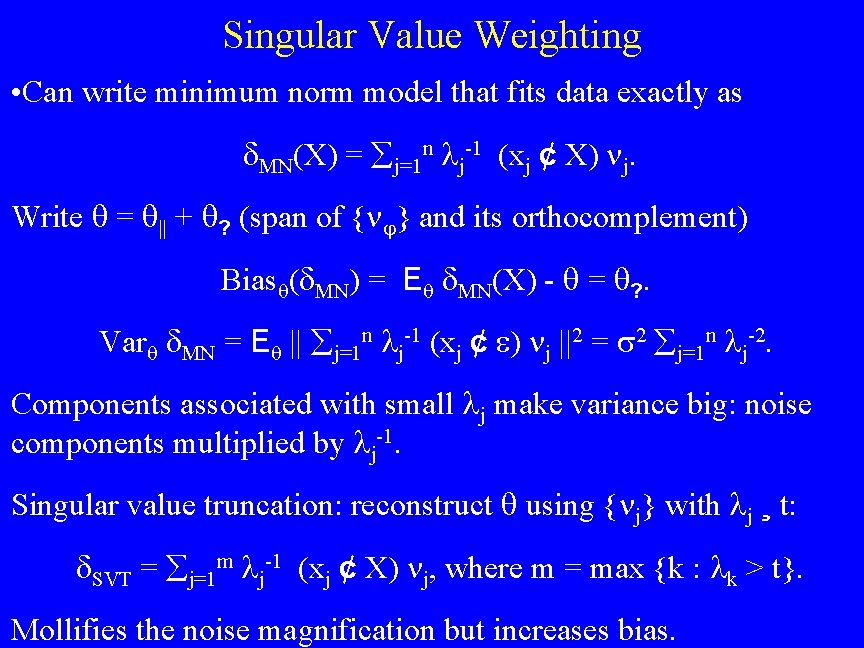
Singular Value Weighting • Can write minimum norm model that fits data exactly as MN(X) = j=1 n j-1 (xj ¢ X) j. Write = || + ? (span of { } and its orthocomplement) Bias ( MN) = E MN(X) - = ? . Var MN = E || j=1 n j-1 (xj ¢ ) j ||2 = 2 j=1 n j-2. Components associated with small j make variance big: noise components multiplied by j-1. Singular value truncation: reconstruct using { j} with j ¸ t: SVT = j=1 m j-1 (xj ¢ X) j, where m = max {k : k > t}. Mollifies the noise magnification but increases bias.

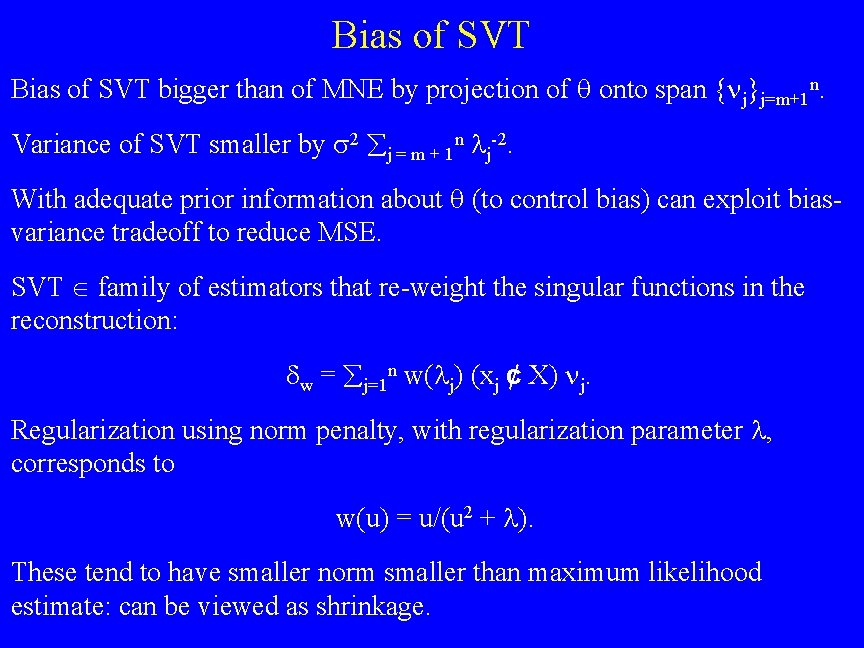
Bias of SVT bigger than of MNE by projection of onto span { j}j=m+1 n. Variance of SVT smaller by 2 j = m + 1 n j-2. With adequate prior information about (to control bias) can exploit biasvariance tradeoff to reduce MSE. SVT family of estimators that re-weight the singular functions in the reconstruction: w = j=1 n w( j) (xj ¢ X) j. Regularization using norm penalty, with regularization parameter , corresponds to w(u) = u/(u 2 + ). These tend to have smaller norm smaller than maximum likelihood estimate: can be viewed as shrinkage.

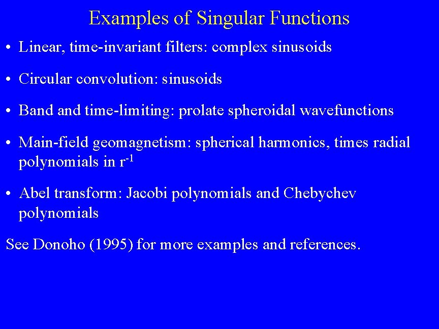
Examples of Singular Functions • Linear, time-invariant filters: complex sinusoids • Circular convolution: sinusoids • Band time-limiting: prolate spheroidal wavefunctions • Main-field geomagnetism: spherical harmonics, times radial polynomials in r-1 • Abel transform: Jacobi polynomials and Chebychev polynomials See Donoho (1995) for more examples and references.

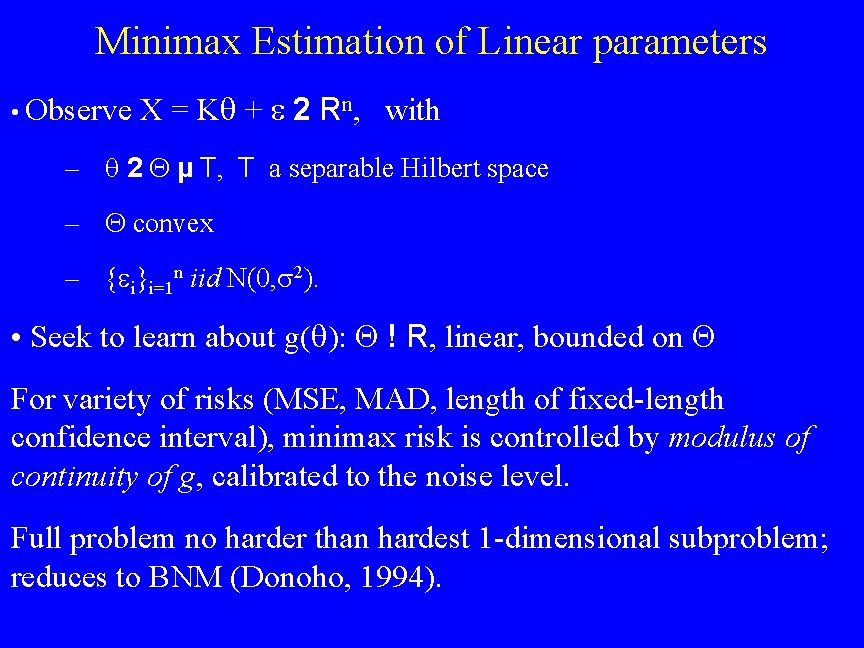
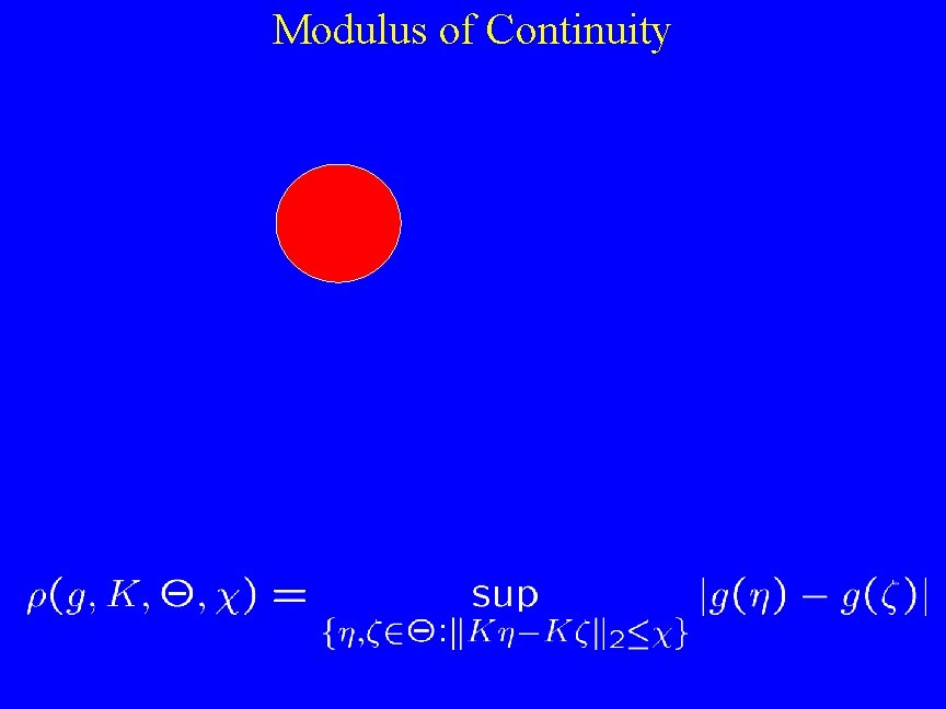
Minimax Estimation of Linear parameters • Observe X = K + 2 Rn, with – 2 µ T, T a separable Hilbert space – convex – { i}i=1 n iid N(0, 2). • Seek to learn about g( ): ! R, linear, bounded on For variety of risks (MSE, MAD, length of fixed-length confidence interval), minimax risk is controlled by modulus of continuity of g, calibrated to the noise level. Full problem no harder than hardest 1 -dimensional subproblem; reduces to BNM (Donoho, 1994).

Example: Geomagnetism = { 2 l 2(w) : l=11 wl m=-ll | lm |2 · q }. Estimate g( ) = lm. Symmetry of and linearity of K, g, let us characterize the modulus: Problem: maximize linear functional of a vector in the intersection of two ellipsoids. In the main-field geomagnetism problem, as the data sampling becomes more uniform over the spherical idealization of a satellite orbit, both the norm (prior information) and the operator K are diagonalized by spherical harmonics.

Modulus of Continuity

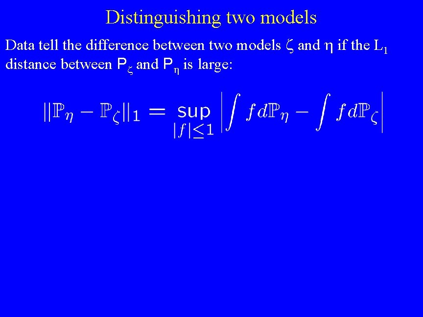
Distinguishing two models Data tell the difference between two models and if the L 1 distance between P and P is large:

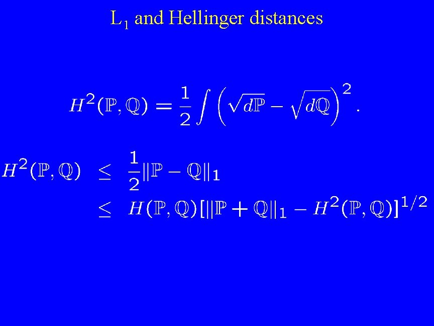
L 1 and Hellinger distances

Consistency in Linear Inverse Problems • Xi = i + i, i=1, 2, 3, … subset of separable Banach space { i} * linear, bounded on { i} iid consistently estimable w. r. t. weak topology iff {Tk}, Tk Borel function of X 1, . . . , Xk, s. t. , >0, *, limk P {| Tk - |> } = 0

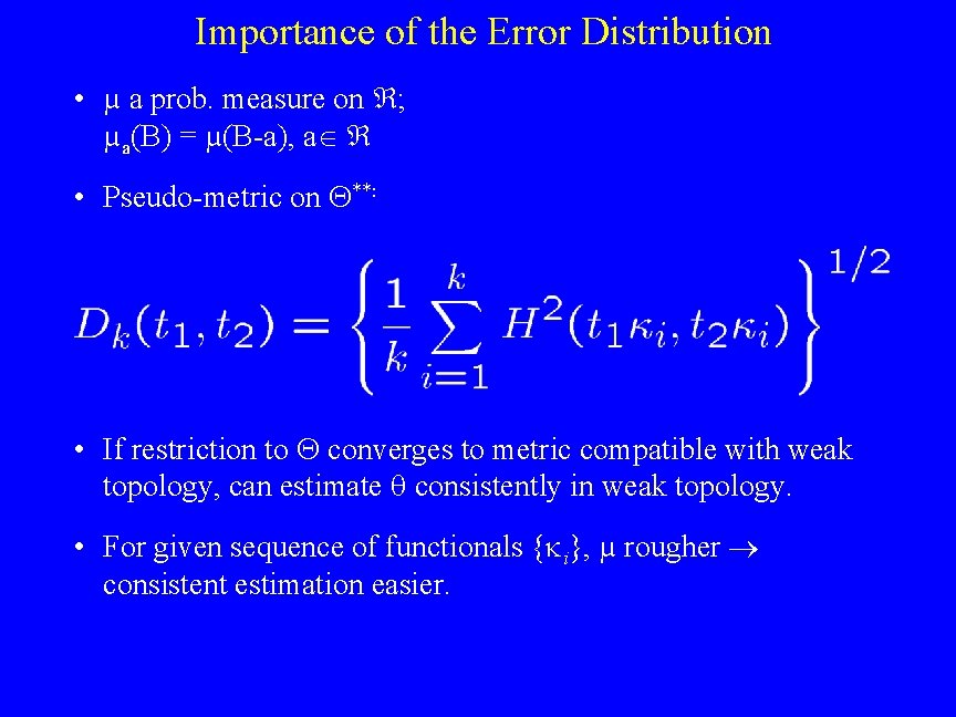
Importance of the Error Distribution • µ a prob. measure on ; µa(B) = µ(B-a), a • Pseudo-metric on **: • If restriction to converges to metric compatible with weak topology, can estimate consistently in weak topology. • For given sequence of functionals { i}, µ rougher consistent estimation easier.

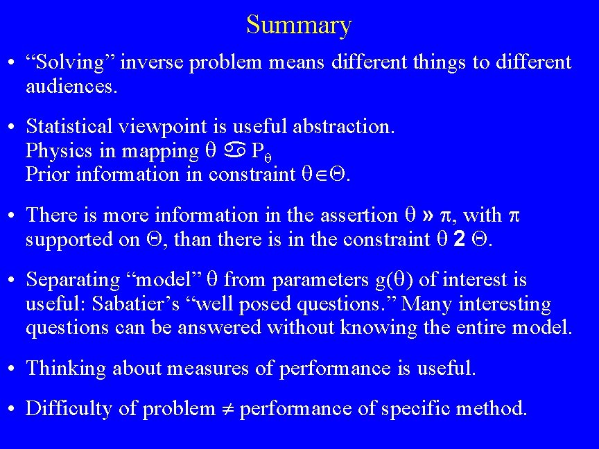
Summary • “Solving” inverse problem means different things to different audiences. • Statistical viewpoint is useful abstraction. Physics in mapping P Prior information in constraint . • There is more information in the assertion » , with supported on , than there is in the constraint 2 • Separating “model” from parameters g( ) of interest is useful: Sabatier’s “well posed questions. ” Many interesting questions can be answered without knowing the entire model. • Thinking about measures of performance is useful. • Difficulty of problem performance of specific method.

References & Acknowledgements Constable, S. C. , R. L. Parker & C. G. Constable, 1987. Occam's inversion: A practical algorithm for generating smooth models from electromagnetic sounding data, Geophysics, 52, 289 -300. Donoho, D. L. , 1994. Statistical Estimation and Optimal Recovery, Ann. Stat. , 22, 238 -270. Donoho, D. L. , 1995. Nonlinear solution of linear inverse problems by wavelet-vaguelette decomposition, Appl. Comput. Harm. Anal. , 2, 101 -126. Evans, S. N. & Stark, P. B. , 2002. Inverse Problems as Statistics, Inverse Problems, 18, R 1 -R 43. Evans, S. N. , B. B. Hansen & P. B. Stark, 2003. Minimax expected measure confidence sets for restricted location parameters, Tech. Rept. 617, Dept. of Statistics, UC Berkeley Le Cam, L. , 1986. Asymptotic Methods in Statistical Decision Theory, Springer-Verlag, NY, 1986, 742 pp. O’Sullivan, F. , 1986. A statistical perspective on ill-posed inverse problems, Statistical Science, 1, 502 -518. Schafer, C. M. & P. B. Stark, 2003. Using what we know: inference with physical constraints, Tech. Rept. , Dept. of Statistics, UC Berkeley Stark, P. B. , 1992. Inference in infinite-dimensional inverse problems: Discretization and duality, J. Geophys. Res. , 97, 14, 055 -14, 082. Stark, P. B. , 1992. Minimax confidence intervals in geomagnetism, Geophys. J. Intl. , 108, 329338.