Quantifying Uncertainty in Belowground Carbon Turnover Ruth D

Quantifying Uncertainty in Belowground Carbon Turnover Ruth D. Yanai State University of New York College of Environmental Science and Forestry Syracuse NY 13210, USA
")
QUANTIFYING UNCERTAINTY IN ECOSYSTEM STUDIES Quantifying uncertainty in ecosystem budgets Precipitation (evaluating monitoring intensity) Streamflow (filling gaps with minimal uncertainty) Forest biomass (identifying the greatest sources of uncertainty) Soil stores, belowground carbon turnover (detectable differences)

Types of uncertainty commonly encountered in ecosystem studies UNCERTAINTY Natural Variability Knowledge Uncertainty Spatial Variability Measurement Error Temporal Variability Model Error Adapted from Harmon et al. (2007)
 Science")
How can we assign confidence in ecosystem nutrient fluxes? Bormann et al. (1977) Science

The N budget for Hubbard Brook published in 1977 was “missing” 14. 2 kg/ha/yr Bormann et al. (1977) Science

The N budget for Hubbard Brook published in 1977 was “missing” 14. 2 kg/ha/yr 14. 2 ± ? ? kg/ha/yr Net N gas exchange = sinks – sources = - precipitation N input + hydrologic export + N accretion in living biomass + N accretion in the forest floor ± gain or loss in soil N stores

The N budget for Hubbard Brook published in 1977 was “missing” 14. 2 kg/ha/yr 14. 2 ± ? ? kg/ha/yr Net N gas exchange = sinks – sources = - precipitation N input + hydrologic export + N accretion in living biomass + N accretion in the forest floor ± gain or loss in soil N stores

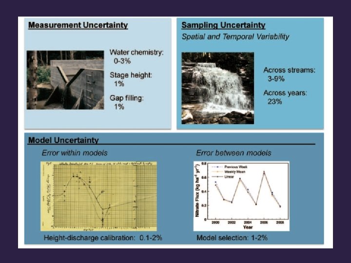
Measurement Uncertainty Sampling Uncertainty Spatial and Temporal Variability Across catchments: 3% Across years: 14% Undercatch: 3. 5% Model Uncertainty Error within models Volume = f(elevation, aspect): 3. 4 mm Error between models Model selection: <1%

We tested the effect of sampling intensity by sequentially omitting individual precipitation gauges. Estimates of annual precipitation volume varied little until five or more of the eleven precipitation gauges were ignored.

The N budget for Hubbard Brook published in 1977 was “missing” 14. 2 kg/ha/yr 14. 2 ± ? ? kg/ha/yr Net N gas exchange = sinks – sources = - precipitation N input (± 1. 3) + hydrologic export + N accretion in living biomass + N accretion in the forest floor ± gain or loss in soil N stores

The N budget for Hubbard Brook published in 1977 was “missing” 14. 2 kg/ha/yr 14. 2 ± ? ? kg/ha/yr Net N gas exchange = sinks – sources = - precipitation N input (± 1. 3) + hydrologic export + N accretion in living biomass + N accretion in the forest floor ± gain or loss in soil N stores

Don Buso HBES

Gaps in the discharge record are filled by comparison to other streams at the site, using linear regression.

Cross-validation: Create fake gaps and compare observed and predicted discharge Gaps of 1 -3 days: <0. 5% Gaps of 1 -2 weeks: ~1% 2 -3 months: 7 -8%

The N budget for Hubbard Brook published in 1977 was “missing” 14. 2 kg/ha/yr 14. 2 ± ? ? kg/ha/yr Net N gas exchange = sinks – sources = - precipitation N input (± 1. 3) + hydrologic export (± 0. 5) + N accretion in living biomass + N accretion in the forest floor ± gain or loss in soil N stores

The N budget for Hubbard Brook published in 1977 was “missing” 14. 2 kg/ha/yr 14. 2 ± ? ? kg/ha/yr Net N gas exchange = sinks – sources = - precipitation N input (± 1. 3) + hydrologic export (± 0. 5) + N accretion in living biomass + N accretion in the forest floor ± gain or loss in soil N stores

Monte Carlo Simulation Monte Carlo simulations use random sampling of the distribution of the inputs to a calculation. After many iterations, the distribution of the output is analyzed. Yanai, Battles, Richardson, Rastetter, Wood, and Blodgett (2010) Ecosystems

A Monte-Carlo approach could be implemented using specialized software or almost any programming language. Here we used a spreadsheet model.

Height Parameters ***IMPORTANT*** Random selection of parameter values happens HERE, not separately for each tree Lookup Height = 10^(a + b*log(Diameter) + log(E))

If the errors were sampled individually for each tree, they would average out to zero by the time you added up a few thousand trees
 + log(E)) PV = 1/2 r")
Biomass Parameters Lookup Biomass = 10^(a + b*log(PV) + log(E)) PV = 1/2 r 2 * Height
 + log(E)) PV = 1/2 r")
Biomass Parameters Lookup Biomass = 10^(a + b*log(PV) + log(E)) PV = 1/2 r 2 * Height
 + log(E)) PV = 1/2 r")
Biomass Parameters Lookup Biomass = 10^(a + b*log(PV) + log(E)) PV = 1/2 r 2 * Height

Concentration Parameters Lookup Concentration = constant + error

COPY THIS ROW-->

Paste Values button After enough interations, analyze your results

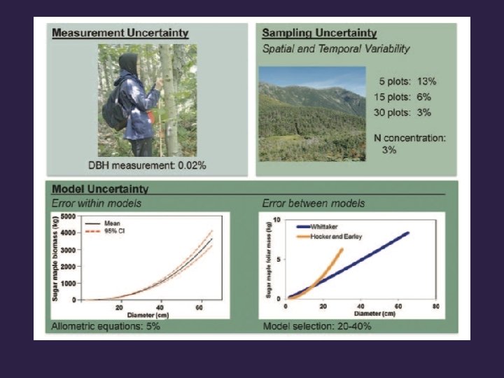
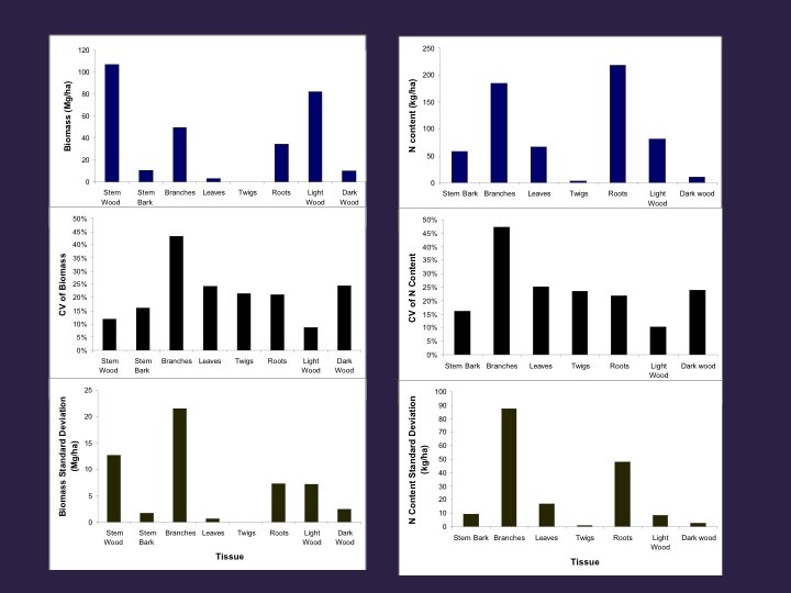
Biomass of thirteen stands of different ages 400 Leaves 350 Branches Bark Wood 300 Biomass (Mg/ha) 250 200 150 100 50 0 C 1 C 2 Young C 3 C 4 C 5 C 6 Mid-Age HB-Mid JB-Mid C 7 C 8 C 9 Old HB- Old JB-Old
 of error in allometric equations 400 3%")
Coefficient of variation (standard deviation / mean) of error in allometric equations 400 3% 2% Leaves 350 4% 4% 5% Branches Bark Wood 300 Biomass (Mg/ha) 250 4% 4% 200 150 3% 7% 3% C 1 C 2 C 3 3% 3% 3% 100 50 0 Young C 4 C 5 C 6 Mid-Age HB-Mid JB-Mid C 7 C 8 C 9 Old HB- Old JB-Old
 Is greater than the uncertainty in the")
CV across plots within stands (spatial variation) Is greater than the uncertainty in the equations 400 16% 10% 19% 3% 2% Leaves 350 4% 3% 4% 11% 5% Branches Bark Wood 300 Biomass (Mg/ha) 250 12% 18% 13% 14% 4% 4% 200 150 3% 3% 3% 6% 15% 11% 3% 7% 3% 100 50 0 C 1 C 2 Young C 3 C 4 C 5 C 6 Mid-Age HB-Mid JB-Mid C 7 C 8 C 9 Old HB- Old JB-Old

“What is the greatest source of uncertainty in my answer? ” Better than the sensitivity estimates that vary everything by the same amount-they don’t all vary by the same amount!

“What is the greatest source of uncertainty to my answer? ” Better than the uncertainty in the parameter estimates--we can tolerate a large uncertainty in an unimportant parameter.

The N budget for Hubbard Brook published in 1977 was “missing” 14. 2 kg/ha/yr 14. 2 ± ? ? kg/ha/yr Net N gas exchange = sinks – sources = - precipitation N input (± 1. 3) + hydrologic export (± 0. 5) + N accretion in living biomass (± 1) + N accretion in the forest floor ± gain or loss in soil N stores

The N budget for Hubbard Brook published in 1977 was “missing” 14. 2 kg/ha/yr 14. 2 ± ? ? kg/ha/yr Net N gas exchange = sinks – sources = - precipitation N input (± 1. 3) + hydrologic export (± 0. 5) + N accretion in living biomass (± 1) + N accretion in the forest floor ± gain or loss in soil N stores

Oi Oe Forest Floor Oa E Bh Bs Mineral Soil

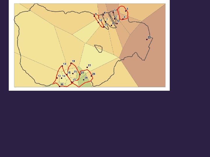
10 points are sampled along each of 5 transects in 13 stands.
")
Excavation of a forest floor block (10 x 10 cm)

• Pin block is trimmed to size. Horizons are easy to see.

• Horizon depths are measured on four faces • Oe, Oi, Oa and A (if present) horizons are bagged separately • In the lab, samples are dried, sieved, and a subsample ovendried for mass and chemical analysis.

Nitrogen in the Forest Floor Hubbard Brook Experimental Forest

Nitrogen in the Forest Floor Hubbard Brook Experimental Forest The change is insignificant (P = 0. 84). The uncertainty in the slope is ± 22 kg/ha/yr.

The N budget for Hubbard Brook published in 1977 was “missing” 14. 2 kg/ha/yr 14. 2 ± ? ? kg/ha/yr Net N gas exchange = sinks – sources = - precipitation N input (± 1. 3) + hydrologic export (± 0. 5) + N accretion in living biomass (± 1) + N accretion in the forest floor (± 22) ± gain or loss in soil N stores

Studies of soil change over time often fail to detect a difference. We should always report how large a difference is detectable. Yanai et al. (2003) SSSAJ

Power analysis can be used to determine the difference detectable with known confidence

Sampling the same experimental units over time permits detection of smaller changes

In this analysis of forest floor studies, few could detect small changes Yanai et al. (2003) SSSAJ

The N budget for Hubbard Brook published in 1977 was “missing” 14. 2 kg/ha/yr 14. 2 ± ? ? kg/ha/yr Net N gas exchange = sinks – sources = - precipitation N input (± 1. 3) + hydrologic export (± 0. 5) + N accretion in living biomass (± 1) + N accretion in the forest floor (± 22) ± gain or loss in soil N stores
 Hubbard Brook Experimental Forest Floor Mineral Soil 10 cm-C Live Vegetation")
Nitrogen Pools (kg/ha) Hubbard Brook Experimental Forest Floor Mineral Soil 10 cm-C Live Vegetation Dead Vegetation Mineral Soil 0 -10 cm Coarse Woody Debris

Quantitative Soil Pits 0. 5 m 2 frame

Excavate Forest Floor by horizon Mineral Soil by depth increment

Sieve and weigh in the field Subsample for laboratory analysis

In some studies, we excavate in the C horizon!

We can’t detect a difference of 730 kg N/ha in the mineral soil. Huntington et al. (1988) From 1983 to 1998, 15 years post-harvest, there was an insignificant decline of 54 ± 53 kg N ha-1 y-1

The N budget for Hubbard Brook published in 1977 was “missing” 14. 2 kg/ha/yr 14. 2 ± ? ? kg/ha/yr Net N gas exchange = sinks – sources = - precipitation N input (± 1. 3) + hydrologic export (± 0. 5) + N accretion in living biomass (± 1) + N accretion in the forest floor (± 22) ± gain or loss in soil N stores (± 53)

The N budget for Hubbard Brook published in 1977 was “missing” 14. 2 kg/ha/yr 14. 2 ± 57 kg/ha/yr Net N gas exchange = sinks – sources = - precipitation N input (± 1. 3) + hydrologic export (± 0. 5) + N accretion in living biomass (± 1) + N accretion in the forest floor (± 22) ± gain or loss in soil N stores (± 53)

Measurement Uncertainty Model Uncertainty Error within models Sampling Uncertainty Spatial Variability Error between models Excludes areas not sampled: rock area 5%, stem area: 1% Measurement uncertainty and spatial variation make it difficult to estimate soil carbon and nutrient contents precisely y

Non-Destructive Evaluation of Soils Neutrons generated by nuclear fusion of 2 H and 3 H interact with nuclei in the soil via inelastic neutron scattering and thermal neutron capture.

TNC INS Agreement with soil pits: 4. 2 vs. 5. 4 kg C m-2. Detectable difference: 5% Time for collection: 1 hour Improvements are needed in portability and sampling geometry. Wielopolski et al. (2010) FEM

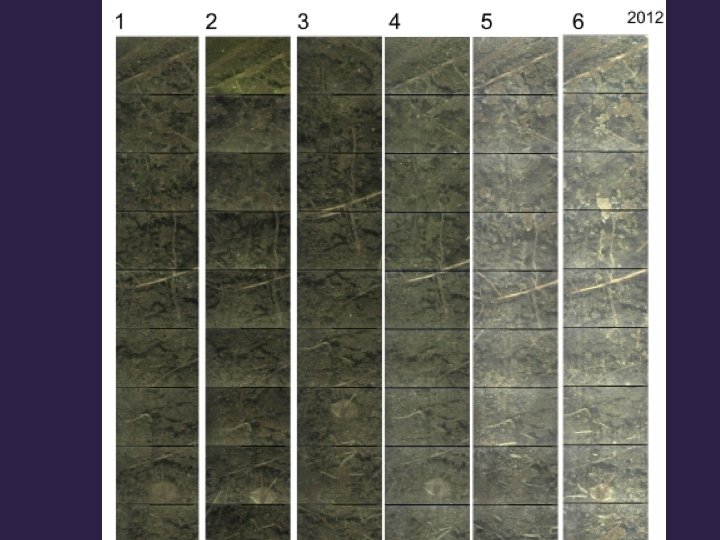
Minirhizotron Estimates of Root Production and Turnover 62

Measurement Uncertainty Sampling Uncertainty Spatial Variability ? Model Uncertainty Root Production vs. Root Lifespan: 45% Park et al. (2003) Ecosystems Sequential Coring, mean vs. max: 30% Brunner al. (2013) Plant Soil

Subjectivity in image analysis could be assessed by multiple observers analyzing the same images

Sources of Uncertainty in Ecosystem Studies Temporal Variation Measurement Spatial Variation Precip Streams Spatial Variation Model uncertainty Model selection Biomass Spatial Variation Soils Measurement Root Turnover Model selection

The Value of Uncertainty Analysis Quantify uncertainty in our results Uncertainty in regression Monte Carlo sampling Detectable differences Identify ways to reduce uncertainty Devote effort to the greatest unknowns Improve efficiency of monitoring efforts

References Yanai, R. D. , C. R. Levine, M. B. Green, and J. L. Campbell. 2012. Quantifying uncertainty in forest nutrient budgets, J. For. 110: 448 -456 Yanai, R. D. , J. J. Battles, A. D. Richardson, E. B. Rastetter, D. M. Wood, and C. Blodgett. 2010. Estimating uncertainty in ecosystem budget calculations. Ecosystems 13: 239 -248 Wielopolski, L, R. D. Yanai, C. R. Levine, S. Mitra, and M. A Vadeboncoeur. 2010. Rapid, non-destructive carbon analysis of forest soils using neutroninduced gamma-ray spectroscopy. For. Ecol. Manag. 260: 1132 -1137 Park, B. B. , R. D. Yanai, T. J. Fahey, T. G. Siccama, S. W. Bailey, J. B. Shanley, and N. L. Cleavitt. 2008. Fine root dynamics and forest production across a calcium gradient in northern hardwood and conifer ecosystems. Ecosystems 11: 325 -341 Yanai, R. D. , S. V. Stehman, M. A. Arthur, C. E. Prescott, A. J. Friedland, T. G. Siccama, and D. Binkley. 2003. Detecting change in forest floor carbon. Soil Sci. Soc. Am. J. 67: 1583 -1593 My web site: www. esf. edu/faculty/yanai (Download any papers)

QUANTIFYING UNCERTAINTY IN ECOSYSTEM STUDIES Be a part of QUEST! • Find more information at: www. quantifyinguncertainty. org • Read papers, share sample code, stay updated with QUEST News • Email us at quantifyinguncertainty@gmail. com • Follow us on Linked. In and Twitter: @QUEST_RCN
- Slides: 69