Quantifying Statistical Control the Threshold of Theoretical Randomization

Quantifying Statistical Control: the Threshold of Theoretical Randomization Kenneth A. Frank Minh Duong Spiro Maroulis Michigan State University Ben Kelcey University of Michigan Presented at Groningen May 21 2008

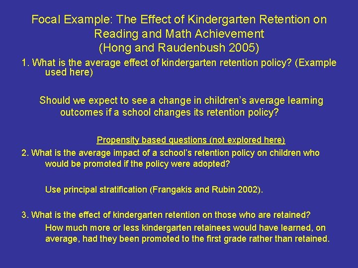
Focal Example: The Effect of Kindergarten Retention on Reading and Math Achievement (Hong and Raudenbush 2005) 1. What is the average effect of kindergarten retention policy? (Example used here) Should we expect to see a change in children’s average learning outcomes if a school changes its retention policy? Propensity based questions (not explored here) 2. What is the average impact of a school’s retention policy on children who would be promoted if the policy were adopted? Use principal stratification (Frangakis and Rubin 2002). 3. What is the effect of kindergarten retention on those who are retained? How much more or less kindergarten retainees would have learned, on average, had they been promoted to the first grade rather than retained.

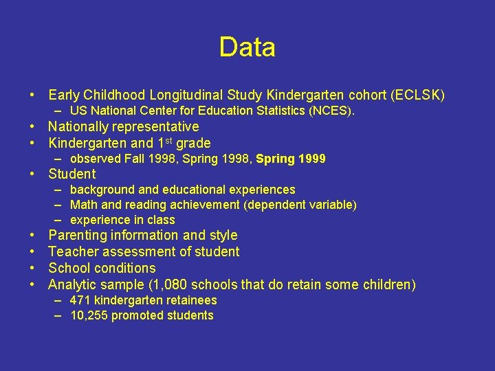
Data • Early Childhood Longitudinal Study Kindergarten cohort (ECLSK) – US National Center for Education Statistics (NCES). • Nationally representative • Kindergarten and 1 st grade – observed Fall 1998, Spring 1999 • Student – background and educational experiences – Math and reading achievement (dependent variable) – experience in class • • Parenting information and style Teacher assessment of student School conditions Analytic sample (1, 080 schools that do retain some children) – 471 kindergarten retainees – 10, 255 promoted students

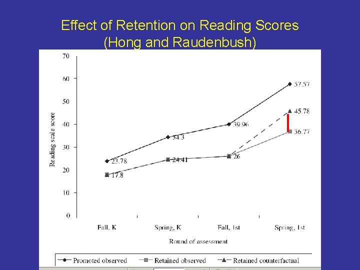
Effect of Retention on Reading Scores (Hong and Raudenbush)

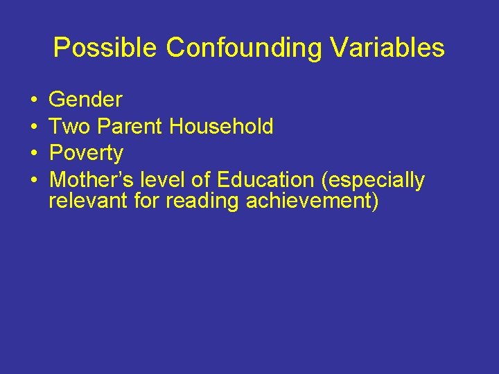
Possible Confounding Variables • • Gender Two Parent Household Poverty Mother’s level of Education (especially relevant for reading achievement)

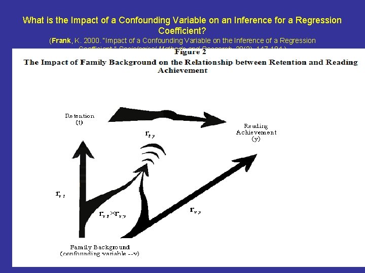
What is the Impact of a Confounding Variable on an Inference for a Regression Coefficient? (Frank, K. 2000. “Impact of a Confounding Variable on the Inference of a Regression Coefficient. ” Sociological Methods and Research, 29(2), 147 -194. )

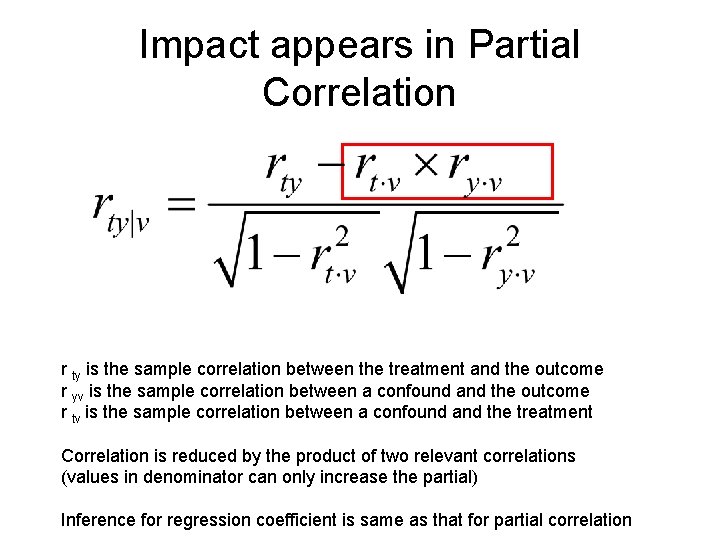
Impact appears in Partial Correlation r ty is the sample correlation between the treatment and the outcome r yv is the sample correlation between a confound and the outcome r tv is the sample correlation between a confound and the treatment Correlation is reduced by the product of two relevant correlations (values in denominator can only increase the partial) Inference for regression coefficient is same as that for partial correlation

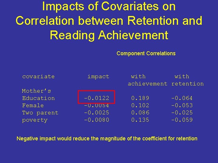
Impacts of Covariates on Correlation between Retention and Reading Achievement Component Correlations covariate impact Mother’s Education Female Two parent poverty -0. 0122 -0. 0054 -0. 0025 -0. 0080 with achievement retention 0. 189 0. 102 0. 086 0. 135 -0. 064 -0. 053 -0. 025 -0. 059 Negative impact would reduce the magnitude of the coefficient for retention

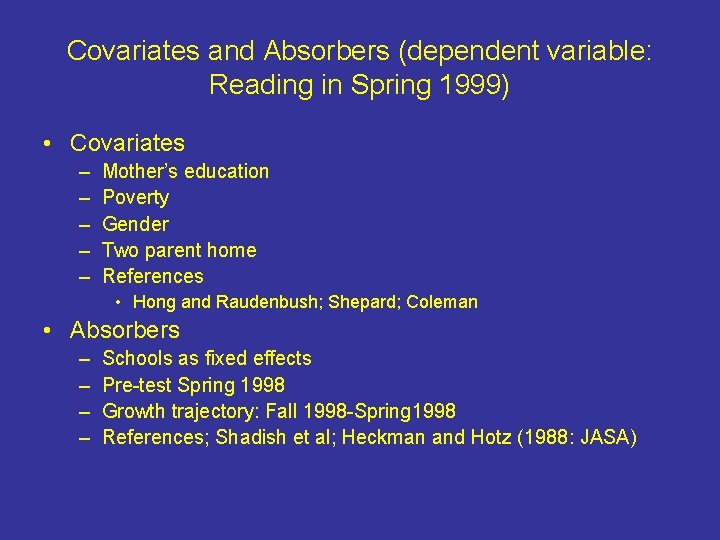
Covariates and Absorbers (dependent variable: Reading in Spring 1999) • Covariates – – – Mother’s education Poverty Gender Two parent home References • Hong and Raudenbush; Shepard; Coleman • Absorbers – – Schools as fixed effects Pre-test Spring 1998 Growth trajectory: Fall 1998 -Spring 1998 References; Shadish et al; Heckman and Hotz (1988: JASA)

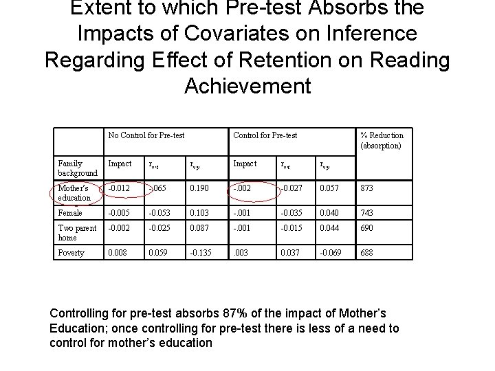
Extent to which Pre-test Absorbs the Impacts of Covariates on Inference Regarding Effect of Retention on Reading Achievement No Control for Pre-test % Reduction (absorption) Family background Impact rv • y Mother’s education -0. 012 -. 065 0. 190 -. 002 -0. 027 0. 057 873 Female -0. 005 -0. 053 0. 103 -. 001 -0. 035 0. 040 743 Two parent home -0. 002 -0. 025 0. 087 -. 001 -0. 015 0. 044 690 Poverty 0. 008 0. 059 -0. 135 . 003 0. 037 -0. 069 688 Controlling for pre-test absorbs 87% of the impact of Mother’s Education; once controlling for pre-test there is less of a need to control for mother’s education

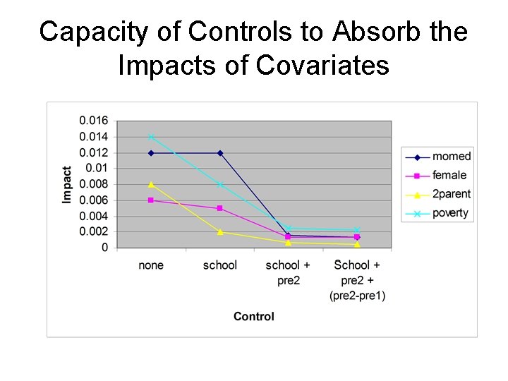
Capacity of Controls to Absorb the Impacts of Covariates

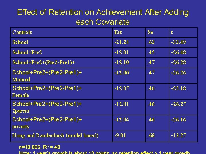
Effect of Retention on Achievement After Adding each Covariate Controls Est Se t School -21. 24 . 63 -33. 49 School+Pre 2 -12. 01 . 45 -26. 48 School+Pre 2+(Pre 2 -Pre 1)+ -12. 10 . 47 -26. 28 School+Pre 2+(Pre 2 -Pre 1)+ Momed -12. 00 . 47 -26. 26 School+Pre 2+(Pre 2 -Pre 1)+ Female -12. 07 . 46 -25. 18 School+Pre 2+(Pre 2 -Pre 1)+ 2 parent -12. 01 . 46 -26. 27 School+Pre 2+(Pre 2 -Pre 1)+ poverty -12. 04 . 46 -26. 16 Hong and Raudenbush (model based) -9. 01 . 68 -13. 27 n=10, 065, R 2 =. 40

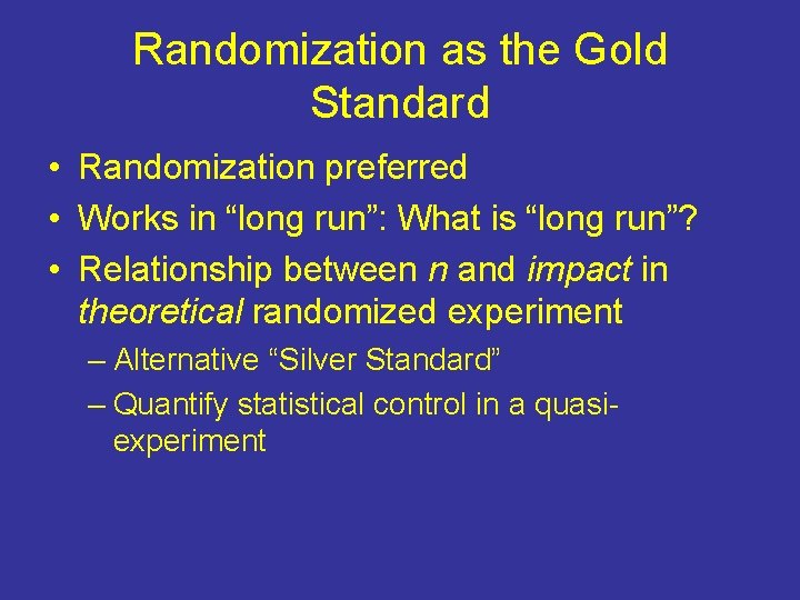
Randomization as the Gold Standard • Randomization preferred • Works in “long run”: What is “long run”? • Relationship between n and impact in theoretical randomized experiment – Alternative “Silver Standard” – Quantify statistical control in a quasiexperiment

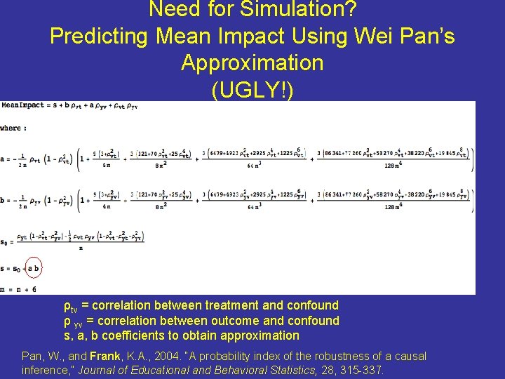
Need for Simulation? Predicting Mean Impact Using Wei Pan’s Approximation (UGLY!) ρtv = correlation between treatment and confound ρ yv = correlation between outcome and confound s, a, b coefficients to obtain approximation Pan, W. , and Frank, K. A. , 2004. “A probability index of the robustness of a causal inference, ” Journal of Educational and Behavioral Statistics, 28, 315 -337.

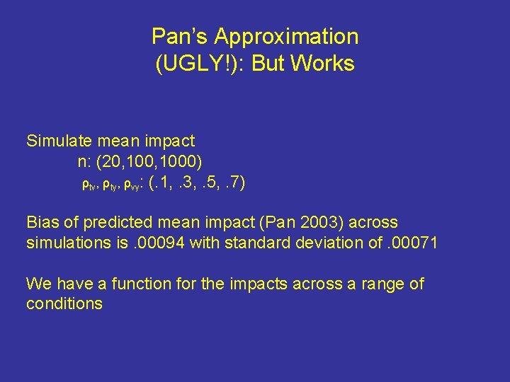
Pan’s Approximation (UGLY!): But Works Simulate mean impact n: (20, 1000) ρtv, ρty, ρvy: (. 1, . 3, . 5, . 7) Bias of predicted mean impact (Pan 2003) across simulations is. 00094 with standard deviation of. 00071 We have a function for the impacts across a range of conditions

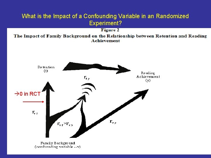
What is the Impact of a Confounding Variable in an Randomized Experiment? 0 in RCT

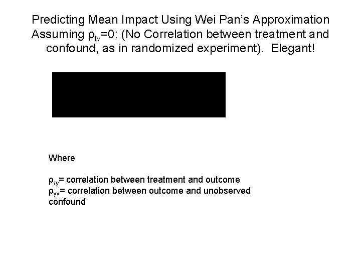
Predicting Mean Impact Using Wei Pan’s Approximation Assuming ρtv=0: (No Correlation between treatment and confound, as in randomized experiment). Elegant! Where ρty= correlation between treatment and outcome ρyv= correlation between outcome and unobserved confound

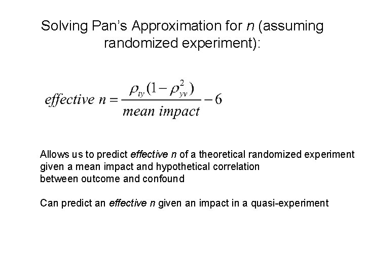
Solving Pan’s Approximation for n (assuming randomized experiment): Allows us to predict effective n of a theoretical randomized experiment given a mean impact and hypothetical correlation between outcome and confound Can predict an effective n given an impact in a quasi-experiment

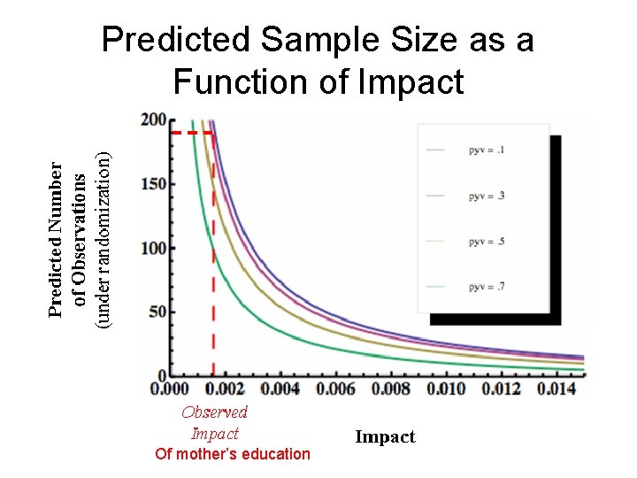
Predicted Sample Size as a Function of Impact Of mother’s education

Quantitative Crosswalk between RCT and Quasi-experiment • Quasi-experiment can achieve same or better level of control as randomized experiment – Red line: Hong and Raudenbush achieve control equivalent to randomized experiment of size 200 better than a small RCT • But, with a randomized experiment – Guaranteed no bias in long run – Confidence interval captures uncertainty • Trade off between precision versus bias – Quasi-experiment could be more precise, but possibly biased – Key assumption: impacts of measured covariates represent impacts of unmeasured covariates.

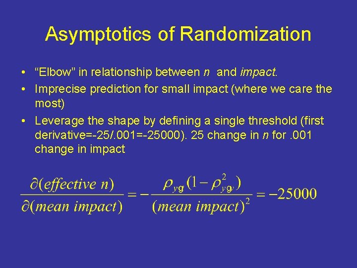
Asymptotics of Randomization • “Elbow” in relationship between n and impact. • Imprecise prediction for small impact (where we care the most) • Leverage the shape by defining a single threshold (first derivative=-25/. 001=-25000). 25 change in n for. 001 change in impact

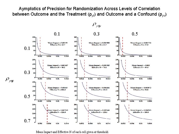
Aymptotics of Precision for Randomization Across Levels of Correlation between Outcome and the Treatment (ρyt) and Outcome and a Confound (ρyv) 0. 1 0. 3 0. 5 0. 7 Mean Impact and Effective N of each cell given at threshold. 0. 5

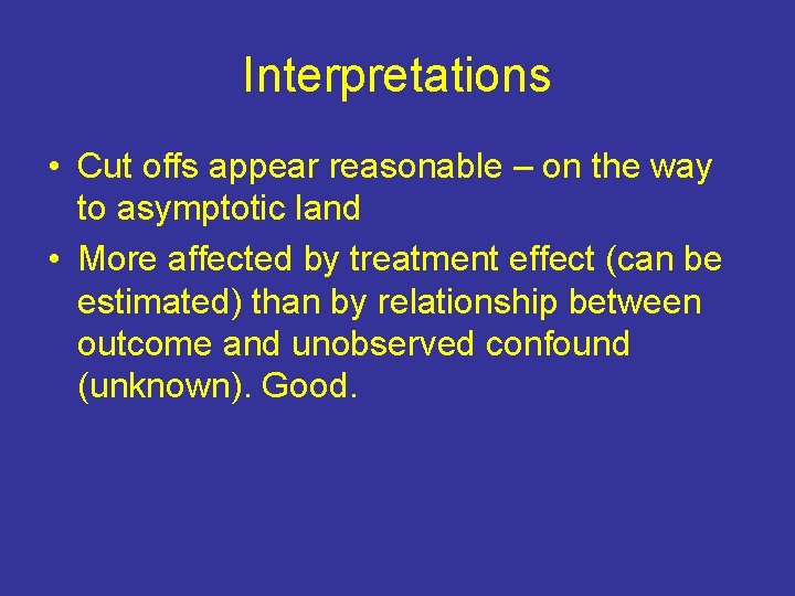
Interpretations • Cut offs appear reasonable – on the way to asymptotic land • More affected by treatment effect (can be estimated) than by relationship between outcome and unobserved confound (unknown). Good.

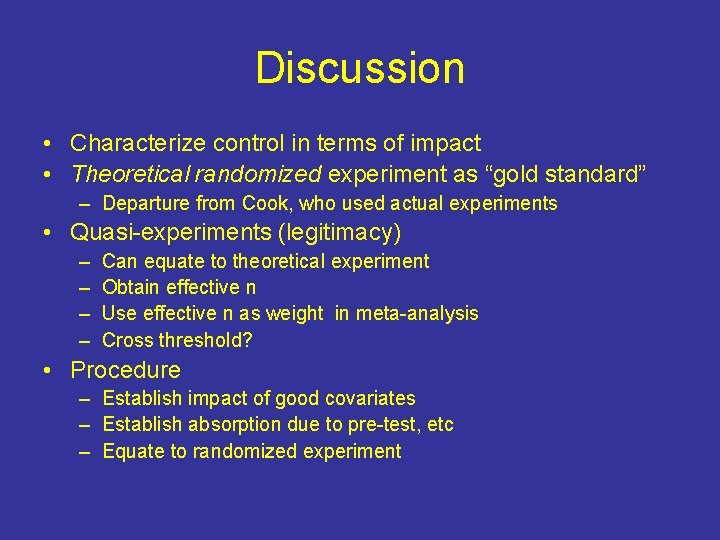
Discussion • Characterize control in terms of impact • Theoretical randomized experiment as “gold standard” – Departure from Cook, who used actual experiments • Quasi-experiments (legitimacy) – – Can equate to theoretical experiment Obtain effective n Use effective n as weight in meta-analysis Cross threshold? • Procedure – Establish impact of good covariates – Establish absorption due to pre-test, etc – Equate to randomized experiment

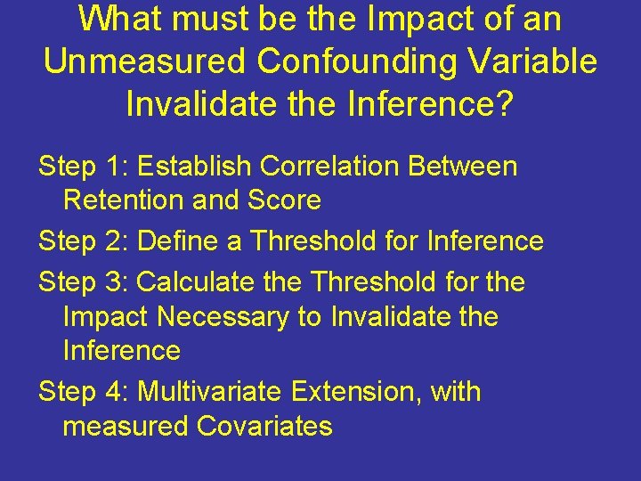
What must be the Impact of an Unmeasured Confounding Variable Invalidate the Inference? Step 1: Establish Correlation Between Retention and Score Step 2: Define a Threshold for Inference Step 3: Calculate the Threshold for the Impact Necessary to Invalidate the Inference Step 4: Multivariate Extension, with measured Covariates

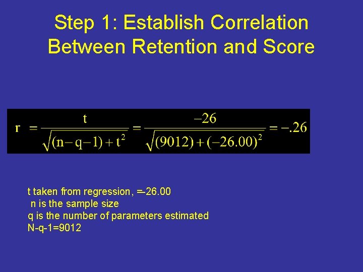
Step 1: Establish Correlation Between Retention and Score t taken from regression, =-26. 00 n is the sample size q is the number of parameters estimated N-q-1=9012

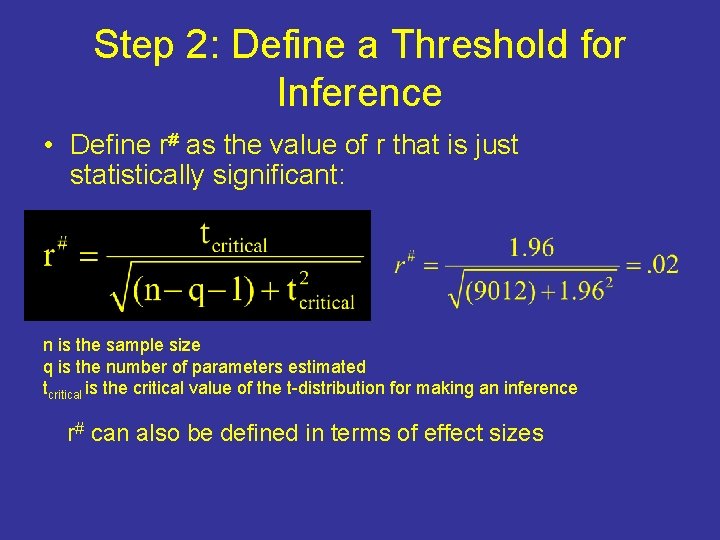
Step 2: Define a Threshold for Inference • Define r# as the value of r that is just statistically significant: n is the sample size q is the number of parameters estimated tcritical is the critical value of the t-distribution for making an inference r# can also be defined in terms of effect sizes

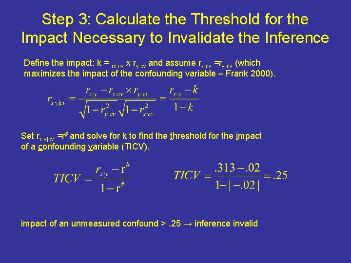
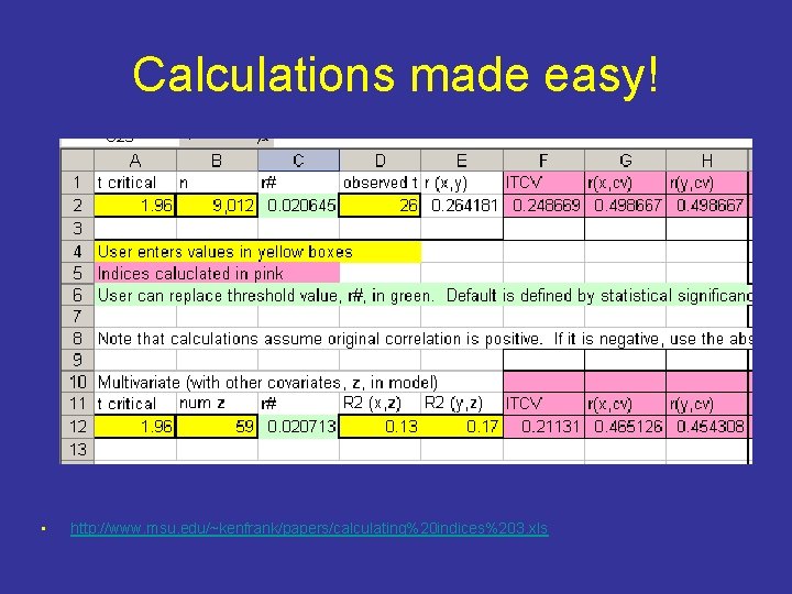
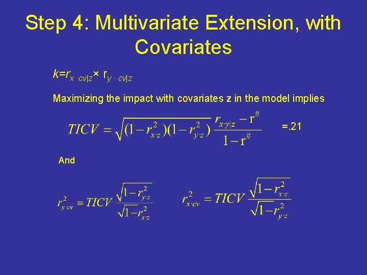
Step 3: Calculate the Threshold for the Impact Necessary to Invalidate the Inference Define the impact: k = rx∙cv x ry∙cv and assume rx∙cv =ry∙cv (which maximizes the impact of the confounding variable – Frank 2000). Set rx∙y|cv =r# and solve for k to find the threshold for the impact of a confounding variable (TICV). impact of an unmeasured confound >. 25 → inference invalid

Calculations made easy! • http: //www. msu. edu/~kenfrank/papers/calculating%20 indices%203. xls

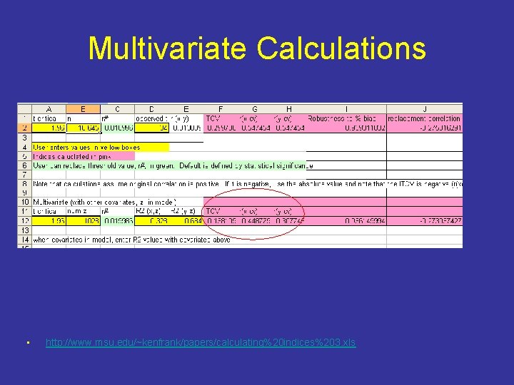
Step 4: Multivariate Extension, with Covariates k=rx ∙cv|z× ry ∙ cv|z Maximizing the impact with covariates z in the model implies =. 21 And

Multivariate Calculations • http: //www. msu. edu/~kenfrank/papers/calculating%20 indices%203. xls

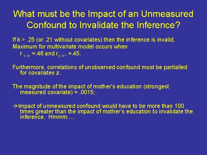
What must be the Impact of an Unmeasured Confound to Invalidate the Inference? If k >. 25 (or. 21 without covariates) then the inference is invalid. Maximum for multivariate model occurs when r x cv =. 46 and ry cv, =. 45. Furthermore, correlations of unobserved confound must be partialled for covariates z. The magnitude of the impact of mother’s education (strongest measured covariate) =. 0015; Impact of unmeasured confound would have to be more than 100 times greater than the impact of mother’s education to invalidate the inference. Hmmm….

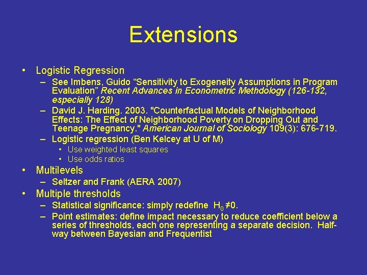
Extensions • Logistic Regression – See Imbens, Guido “Sensitivity to Exogeneity Assumptions in Program Evaluation” Recent Advances in Econometric Methdology (126 -132, especially 128) – David J. Harding. 2003. "Counterfactual Models of Neighborhood Effects: The Effect of Neighborhood Poverty on Dropping Out and Teenage Pregnancy. " American Journal of Sociology 109(3): 676 -719. – Logistic regression (Ben Kelcey at U of M) • Use weighted least squares • Use odds ratios • Multilevels – Seltzer and Frank (AERA 2007) • Multiple thresholds – Statistical significance: simply redefine H 0 ≠ 0. – Point estimates: define impact necessary to reduce coefficient below a series of thresholds, each one representing a separate decision. Halfway between Bayesian and Frequentist

Actual Randomized Experiment • • Effect of Technology on Teaching Strong Methods Randomization Still some Confounding

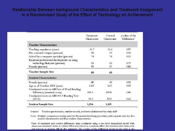
Relationship Between background Characteristics and Treatment Assignment in a Randomized Study of the Effect of Technology on Achievement