Quantifying Natural Selection using Hyphy Reporter Chen Wenjun

Quantifying Natural Selection using Hyphy Reporter : Chen Wenjun from LMSE, Shanghai Ocean University, Shanghai, China

Natural Selection • Mutation, recombination and other processes introduce variation into genomes of organisms. • The fitness of an organism describes how well it can survive or grow in a given environment, or how well it can pass on its genetic material to future generations. • Any mutation can be • Neutral: no or little change in fitness • Deleterious: reduced fitness • Adaptive: increased fitness. • The same mutation can have different fitness costs in different environments (fitness landscape), and different genetic backgrounds (epistasis).

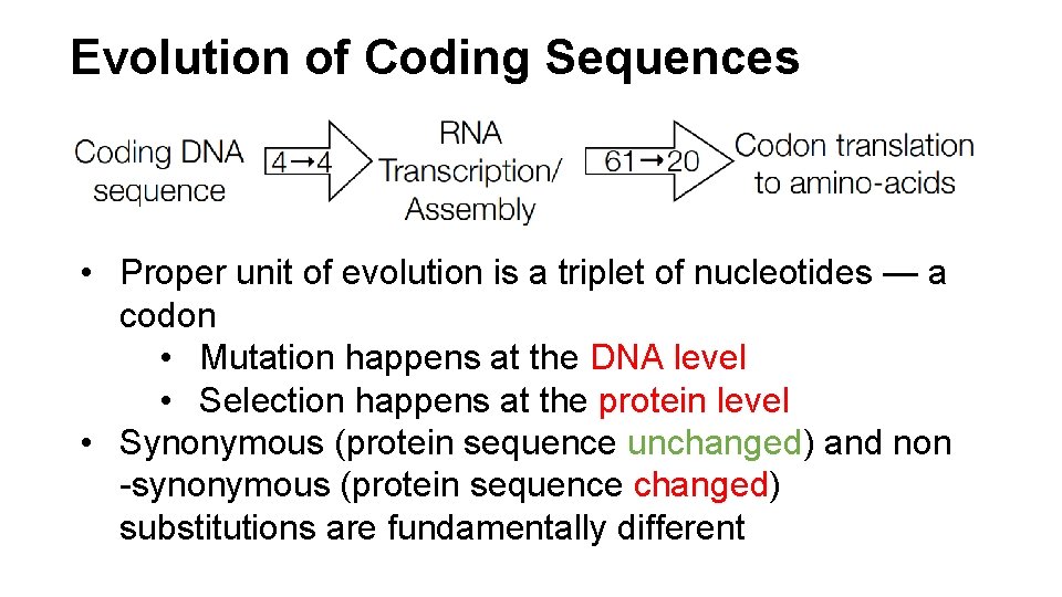
Evolution of Coding Sequences • Proper unit of evolution is a triplet of nucleotides — a codon • Mutation happens at the DNA level • Selection happens at the protein level • Synonymous (protein sequence unchanged) and non -synonymous (protein sequence changed) substitutions are fundamentally different

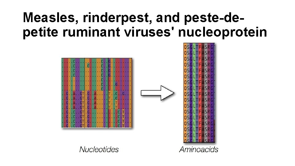
Measles, rinderpest, and peste-depetite ruminant viruses' nucleoprotein

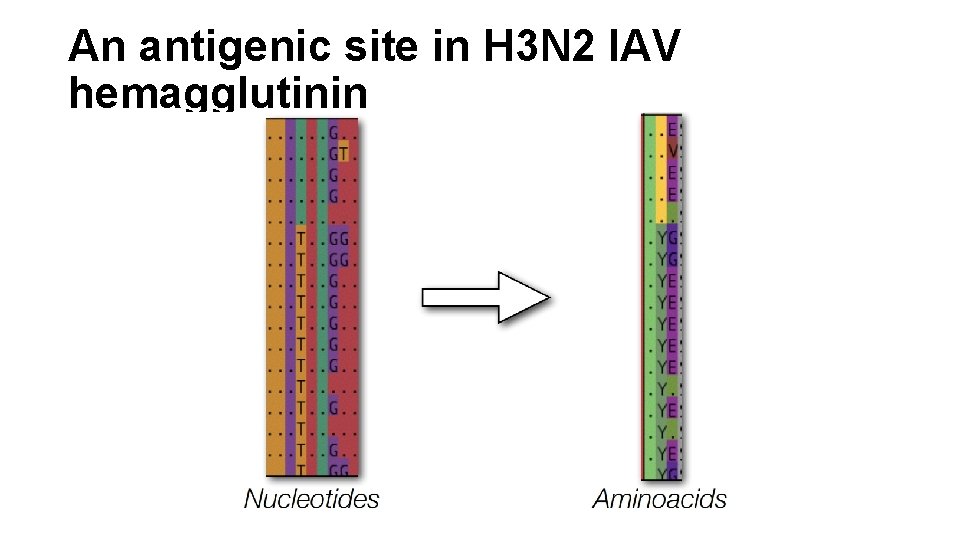
An antigenic site in H 3 N 2 IAV hemagglutinin

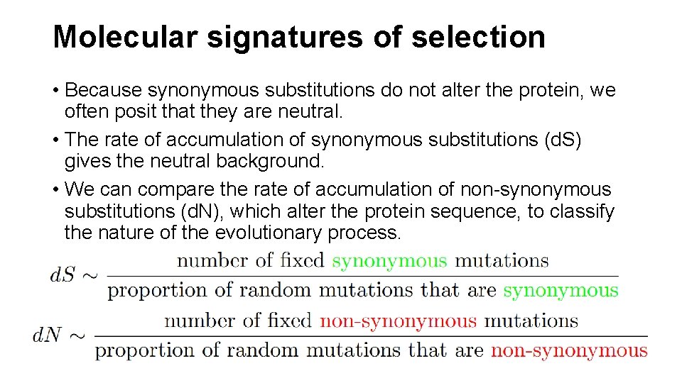
Molecular signatures of selection • Because synonymous substitutions do not alter the protein, we often posit that they are neutral. • The rate of accumulation of synonymous substitutions (d. S) gives the neutral background. • We can compare the rate of accumulation of non-synonymous substitutions (d. N), which alter the protein sequence, to classify the nature of the evolutionary process.

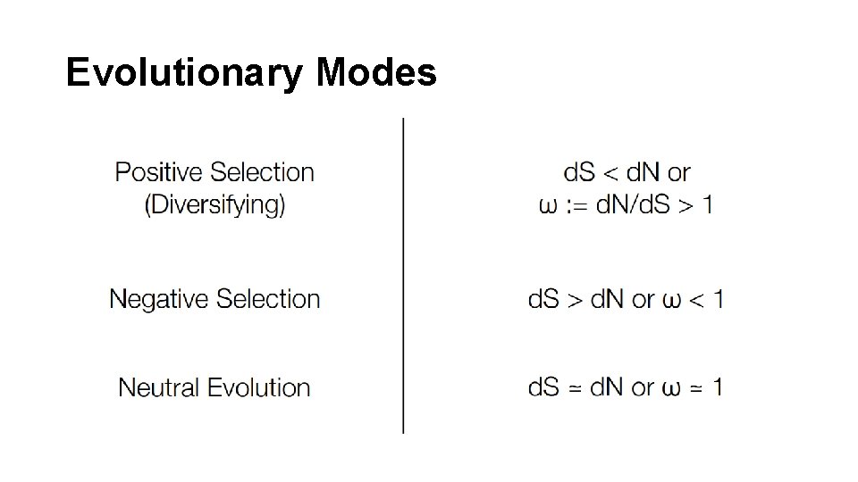
Evolutionary Modes

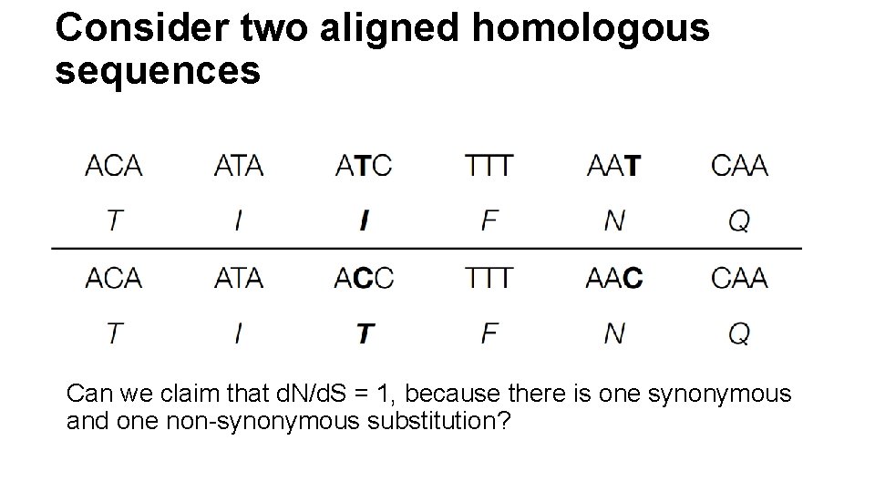
Consider two aligned homologous sequences Can we claim that d. N/d. S = 1, because there is one synonymous and one non-synonymous substitution?

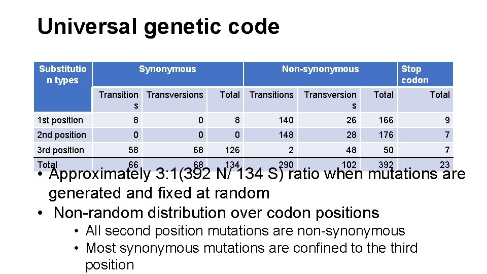
Universal genetic code Substitutio n types Synonymous Non-synonymous Transition Transversions s Total Transitions Stop codon Transversion s Total 1 st position 8 0 8 140 26 166 9 2 nd position 0 0 0 148 28 176 7 3 rd position 58 68 126 2 48 50 7 Total 66 68 134 290 102 392 23 • Approximately 3: 1(392 N/ 134 S) ratio when mutations are generated and fixed at random • Non-random distribution over codon positions • All second position mutations are non-synonymous • Most synonymous mutations are confined to the third position

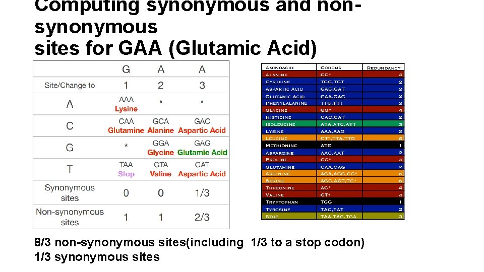
Computing synonymous and nonsynonymous sites for GAA (Glutamic Acid) 8/3 non-synonymous sites(including 1/3 to a stop codon) 1/3 synonymous sites

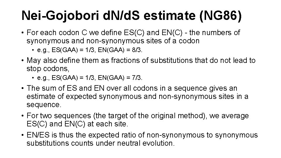
Nei-Gojobori d. N/d. S estimate (NG 86) • For each codon C we define ES(C) and EN(C) - the numbers of synonymous and non-synonymous sites of a codon • e. g. , ES(GAA) = 1/3, EN(GAA) = 8/3. • May also define them as fractions of substitutions that do not lead to stop codons, • e. g. , ES(GAA) = 1/3, EN(GAA) = 7/3. • The sum of ES and EN over all codons in a sequence gives an estimate of expected synonymous and non-synonymous sites in a sequence. • For two sequences (the target of the original method), we average ES(C) and EN(C) at each site. • EN/ES is thus the expected ratio of non-synonymous to synonymous substitutions counts under neutral evolution.

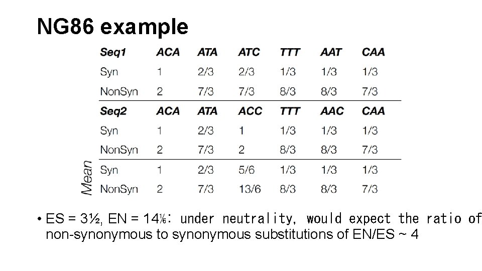
NG 86 example • ES = 3½, EN = 14⅙: under neutrality, would expect the ratio of non-synonymous to synonymous substitutions of EN/ES ~ 4

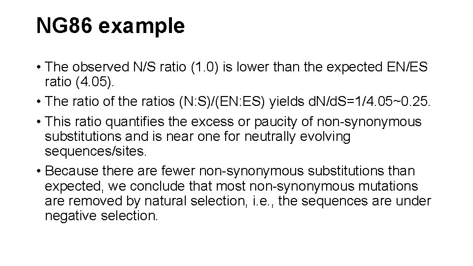
NG 86 example • The observed N/S ratio (1. 0) is lower than the expected EN/ES ratio (4. 05). • The ratio of the ratios (N: S)/(EN: ES) yields d. N/d. S=1/4. 05~0. 25. • This ratio quantifies the excess or paucity of non-synonymous substitutions and is near one for neutrally evolving sequences/sites. • Because there are fewer non-synonymous substitutions than expected, we conclude that most non-synonymous mutations are removed by natural selection, i. e. , the sequences are under negative selection.

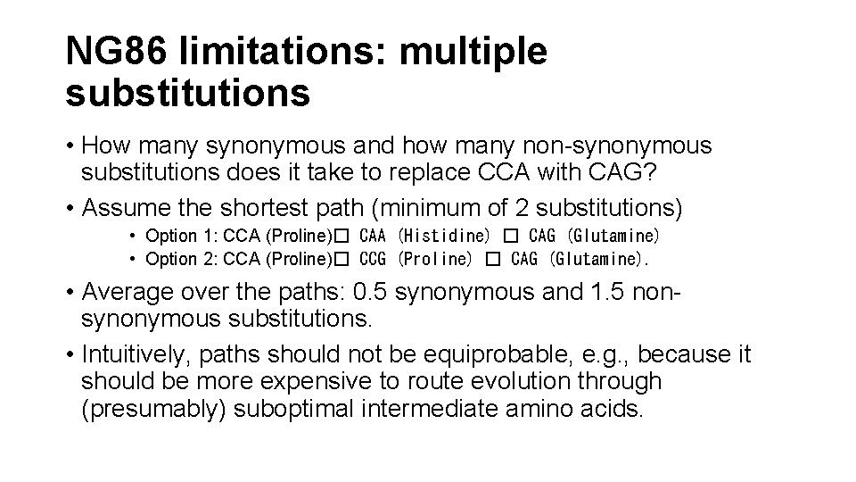
NG 86 limitations: multiple substitutions • How many synonymous and how many non-synonymous substitutions does it take to replace CCA with CAG? • Assume the shortest path (minimum of 2 substitutions) • Option 1: CCA (Proline)� CAA (Histidine) � CAG (Glutamine) • Option 2: CCA (Proline)� CCG (Proline) � CAG (Glutamine). • Average over the paths: 0. 5 synonymous and 1. 5 nonsynonymous substitutions. • Intuitively, paths should not be equiprobable, e. g. , because it should be more expensive to route evolution through (presumably) suboptimal intermediate amino acids.

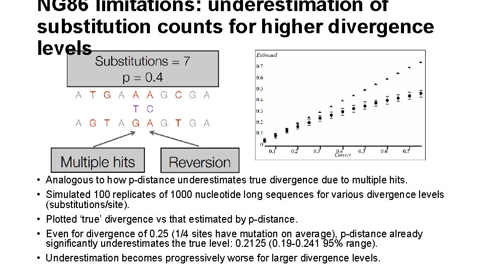
NG 86 limitations: underestimation of substitution counts for higher divergence levels • Analogous to how p-distance underestimates true divergence due to multiple hits. • Simulated 100 replicates of 1000 nucleotide long sequences for various divergence levels (substitutions/site). • Plotted ‘true’ divergence vs that estimated by p-distance. • Even for divergence of 0. 25 (1/4 sites have mutation on average), p-distance already significantly underestimates the true level: 0. 2125 (0. 19 -0. 241 95% range). • Underestimation becomes progressively worse for larger divergence levels.

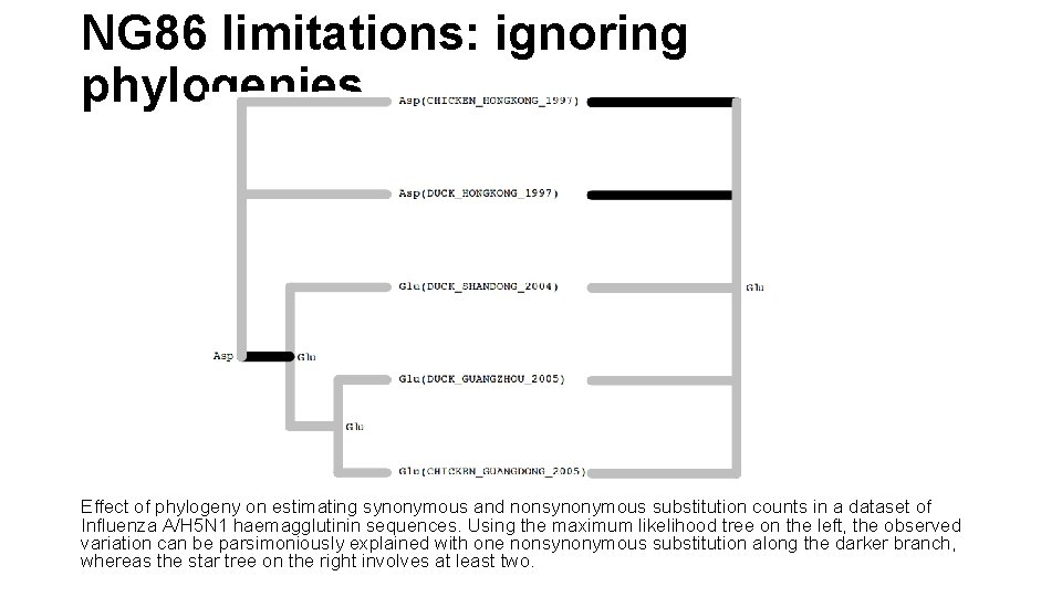
NG 86 limitations: ignoring phylogenies Effect of phylogeny on estimating synonymous and nonsynonymous substitution counts in a dataset of Influenza A/H 5 N 1 haemagglutinin sequences. Using the maximum likelihood tree on the left, the observed variation can be parsimoniously explained with one nonsynonymous substitution along the darker branch, whereas the star tree on the right involves at least two.

NG 86 limitations: averaging across all sites in a gene • Different sites in a gene will be subject to different selective forces • A gene-wide measure of selection is going to average these effects • Most sites in most genes will be maintained by purifying selection • Positively selected sites are of great biological interest, because they point to how a particular gene can respond to selective pressures • Negatively selected sites are also of interest, because they point to functional constraint, and could be used to guide drug or vaccine design • Must develop methods that are able to disentangle the contributions of individual sites

Codon-substitution models • In 1994, first tractable mechanistic evolutionary models for codon sequences were proposed by Muse and Gaut (MG 94), and, independently, by Goldman and Yang (GY 94) [in the same issue of MBE, back to back] • Markov models of codon substitution provide a powerful framework for estimating substitution rates from coding sequence data, as they • • encode our mechanistic understanding of the evolutionary process, enable one to compute phylogenetic likelihood, permit Hypothesis testing or Bayesian inference, systematically account for confounding processes (unequal base frequencies, nucleotide substitution biases, etc. ), • afford many opportunities for extension and refinement (still happening today).

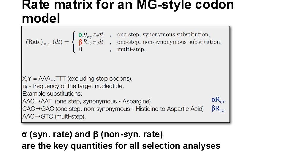
Rate matrix for an MG-style codon model α (syn. rate) and β (non-syn. rate) are the key quantities for all selection analyses

Computing the transition probabilities • In order to recover transition probabilities T(t) from the rate matrix Q, one computes the matrix exponential T(t) = exp (Qt, same as with standard nucleotide models, e. g. HKY 85 or GTR) • Because the computational complexity of matrix exponentiation scales as the cube of the matrix dimension, codon based models require roughly (61/4)3 ≈ 3500 more operations than nucleotide models • This explains why codon probabilistic models were not introduced until the 1990 s, even though they are straightforward extensions of 4 x 4 nucleotide models

Multiple substitutions • The model assumes that point mutations alter one nucleotide at a time, hence most of the instantaneous rates (3134/3761 or 84. 2% in the case of the universal genetic code) are 0. • This restriction, however, does not mean that the model disallows any substitutions that involve multiple nucleotides (e. g. , ACT�AGG). • Such substitutions must simply be realized via several single nucleotide steps, e. g. ACT�AGG • In fact the (i, j) element of T(t) = exp(Qt) sums the probabilities of all such possible pathways of duration t, including reversions

Alignment-wide estimates • Using standard Maximum Likelihood Estimate(MLE) approaches it is straightforward to obtain point estimates of d. N/d. S : = β/α • Can also easily test whether or not d. N/d. S > 1, or < 1 using the likelihood ratio test (LRT) • Codon models also support the concepts of synonymous and nonsynonymous distances between sequences using standard properties of Markov processes (exponentially distributed waiting times)

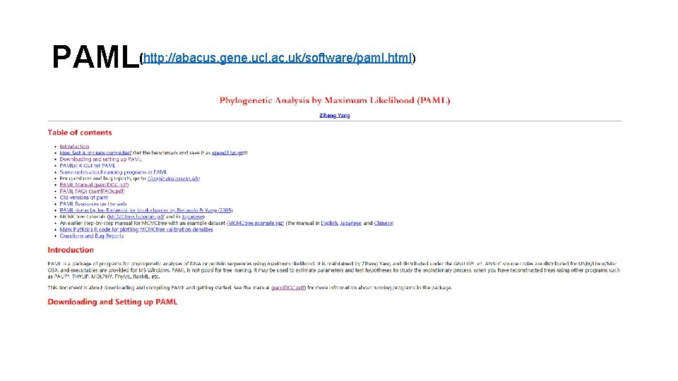
PAML(http: //abacus. gene. ucl. ac. uk/software/paml. html)

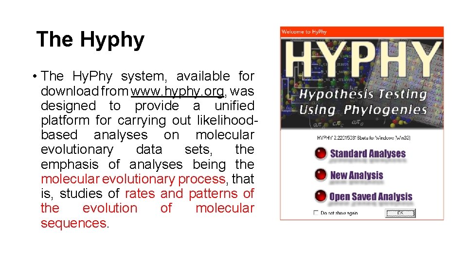
The Hyphy • The Hy. Phy system, available for download from www. hyphy. org, was designed to provide a unified platform for carrying out likelihoodbased analyses on molecular evolutionary data sets, the emphasis of analyses being the molecular evolutionary process, that is, studies of rates and patterns of the evolution of molecular sequences.

Getting Started with Hy. Phy

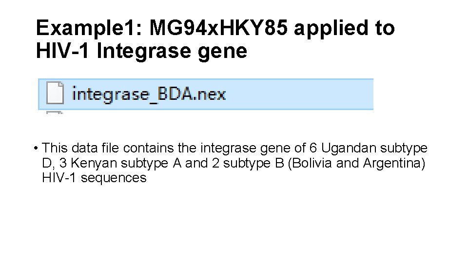
Example 1: MG 94 x. HKY 85 applied to HIV-1 Integrase gene • This data file contains the integrase gene of 6 Ugandan subtype D, 3 Kenyan subtype A and 2 subtype B (Bolivia and Argentina) HIV-1 sequences

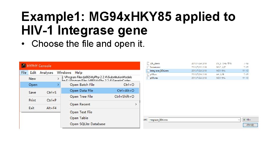
Example 1: MG 94 x. HKY 85 applied to HIV-1 Integrase gene • Choose the file and open it.

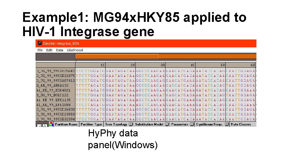
Example 1: MG 94 x. HKY 85 applied to HIV-1 Integrase gene Hy. Phy data panel(Windows)

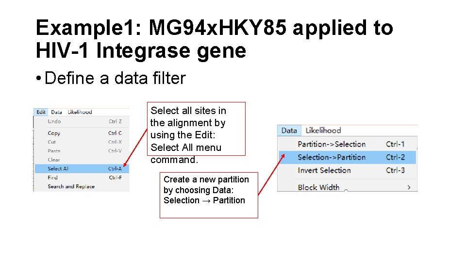
Example 1: MG 94 x. HKY 85 applied to HIV-1 Integrase gene • Define a data filter Select all sites in the alignment by using the Edit: Select All menu command. Create a new partition by choosing Data: Selection → Partition

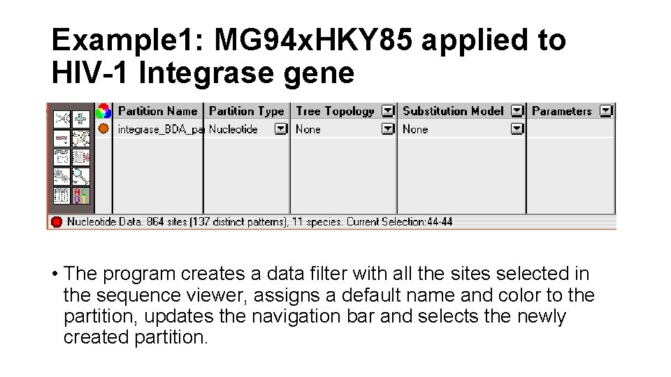
Example 1: MG 94 x. HKY 85 applied to HIV-1 Integrase gene • The program creates a data filter with all the sites selected in the sequence viewer, assigns a default name and color to the partition, updates the navigation bar and selects the newly created partition.

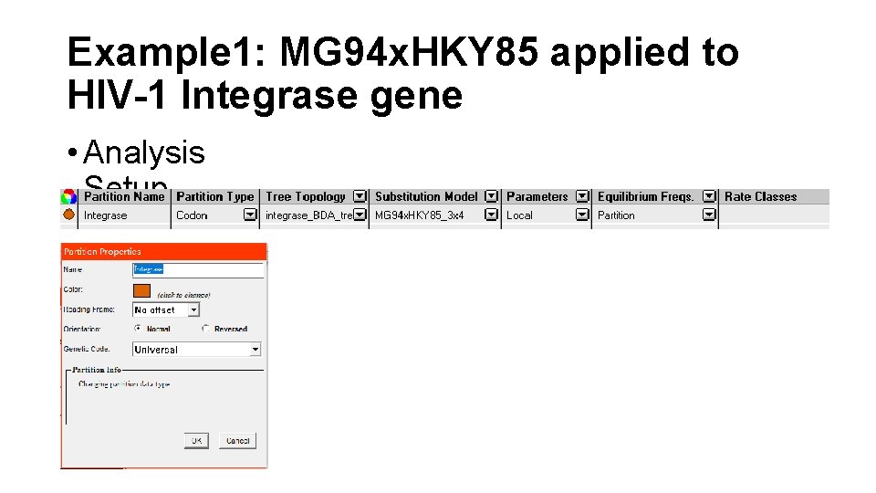
Example 1: MG 94 x. HKY 85 applied to HIV-1 Integrase gene • Analysis Setup

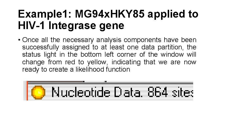
Example 1: MG 94 x. HKY 85 applied to HIV-1 Integrase gene • Once all the necessary analysis components have been successfully assigned to at least one data partition, the status light in the bottom left corner of the window will change from red to yellow, indicating that we are now ready to create a likelihood function

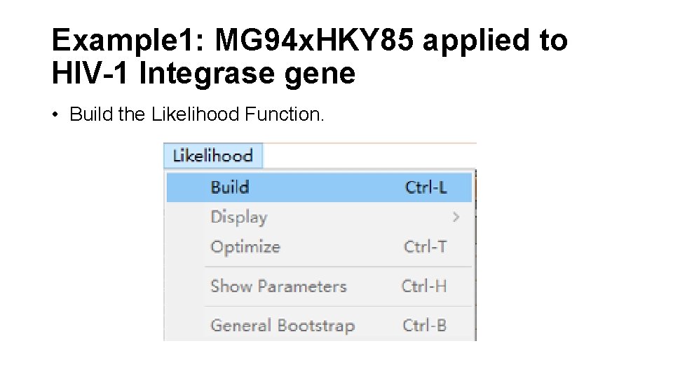
Example 1: MG 94 x. HKY 85 applied to HIV-1 Integrase gene • Build the Likelihood Function.

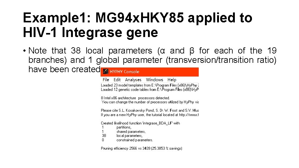
Example 1: MG 94 x. HKY 85 applied to HIV-1 Integrase gene • Note that 38 local parameters (α and β for each of the 19 branches) and 1 global parameter (transversion/transition ratio) have been created.

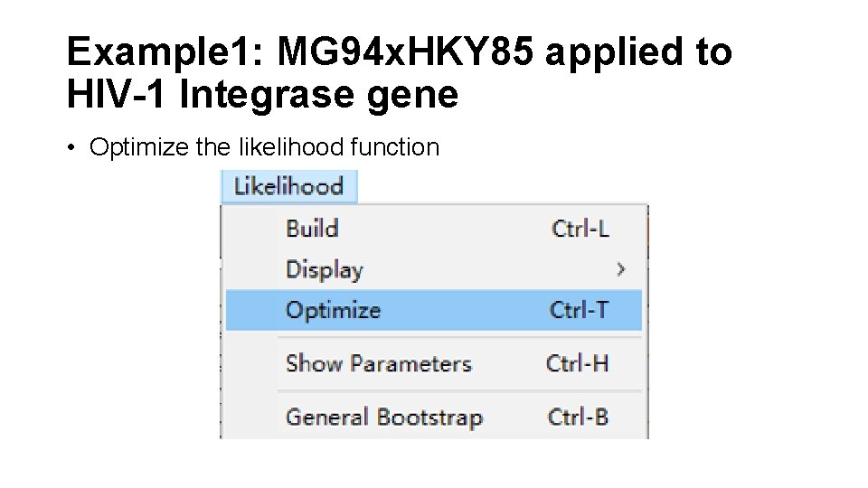
Example 1: MG 94 x. HKY 85 applied to HIV-1 Integrase gene • Optimize the likelihood function

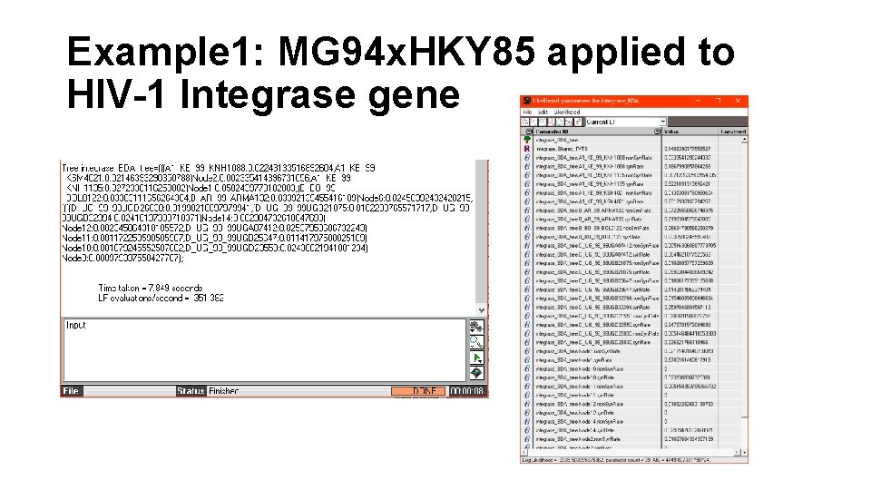
Example 1: MG 94 x. HKY 85 applied to HIV-1 Integrase gene

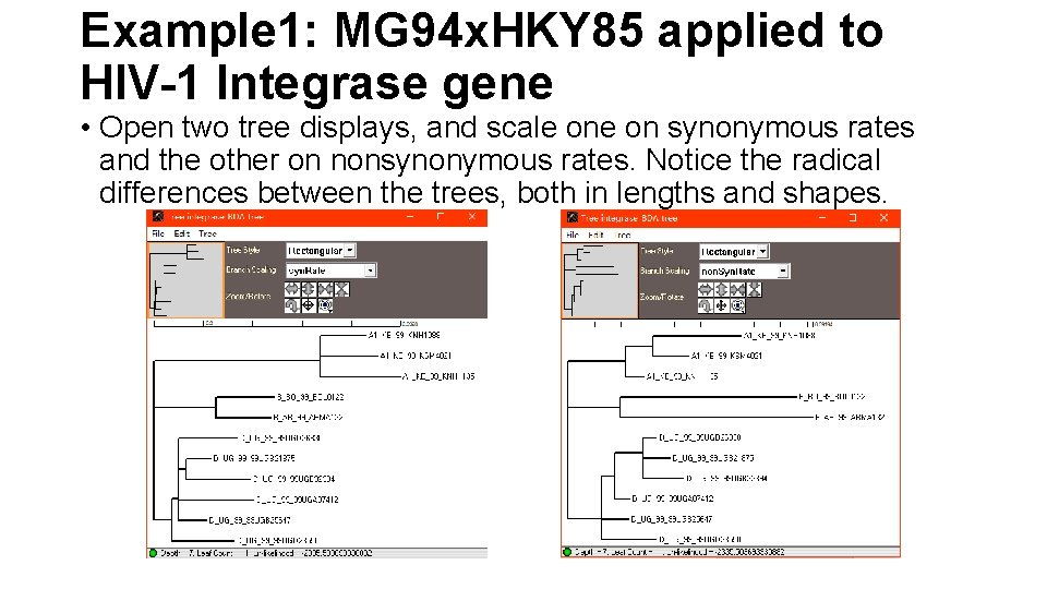
Example 1: MG 94 x. HKY 85 applied to HIV-1 Integrase gene • Open two tree displays, and scale on synonymous rates and the other on nonsynonymous rates. Notice the radical differences between the trees, both in lengths and shapes.

Example 2: Spatial Rate Heterogeneity: Selective Pressure and Functional Constraints • In this example we allow both synonymous and nonsynonymous rates to be variable across sites, leading to the possibility, for instance, that a particular site might have a fast nonsynonymous rate but a slow synonymous rate. We will consider the case of MG 94 x. HKY 85 applied to a codon data set with αs and βs sampled independently from two separate distributions. Because only products of evolutionary rates and times can be estimated, we let the mean of the distribution of αs to be one. Widely used models of Nielsen and Yang (1998) assume that αs = 1 for every site s, thus our approach is a natural extension.

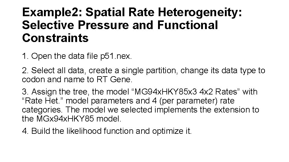
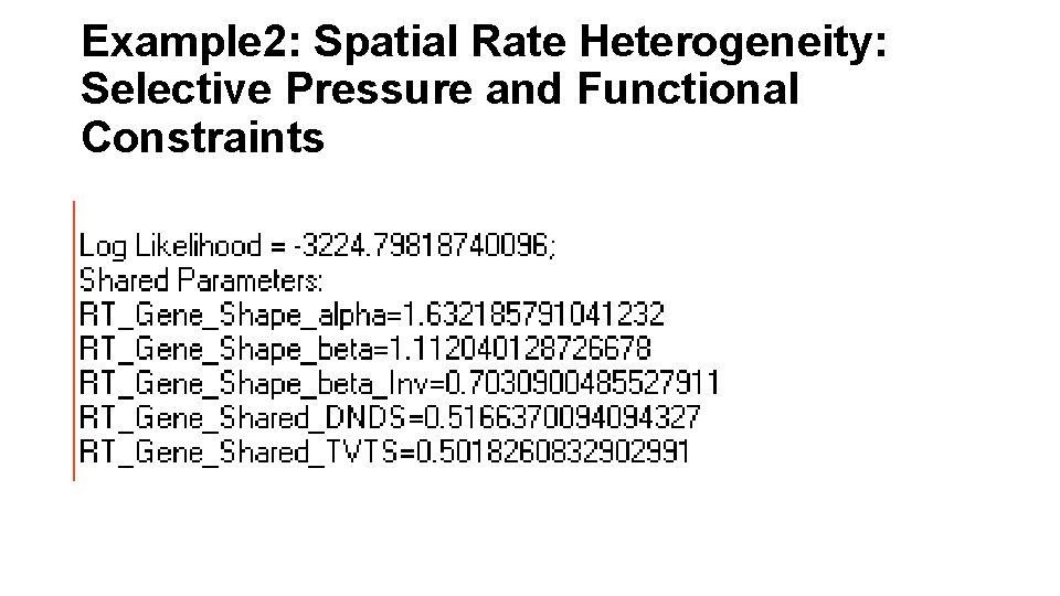
Example 2: Spatial Rate Heterogeneity: Selective Pressure and Functional Constraints 1. Open the data file p 51. nex. 2. Select all data, create a single partition, change its data type to codon and name to RT Gene. 3. Assign the tree, the model “MG 94 x. HKY 85 x 3 4 x 2 Rates” with “Rate Het. ” model parameters and 4 (per parameter) rate categories. The model we selected implements the extension to the MGx 94 x. HKY 85 model. 4. Build the likelihood function and optimize it.

Example 2: Spatial Rate Heterogeneity: Selective Pressure and Functional Constraints

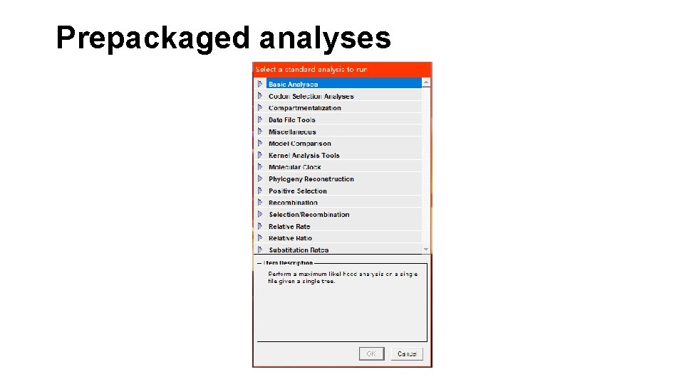
Prepackaged analyses

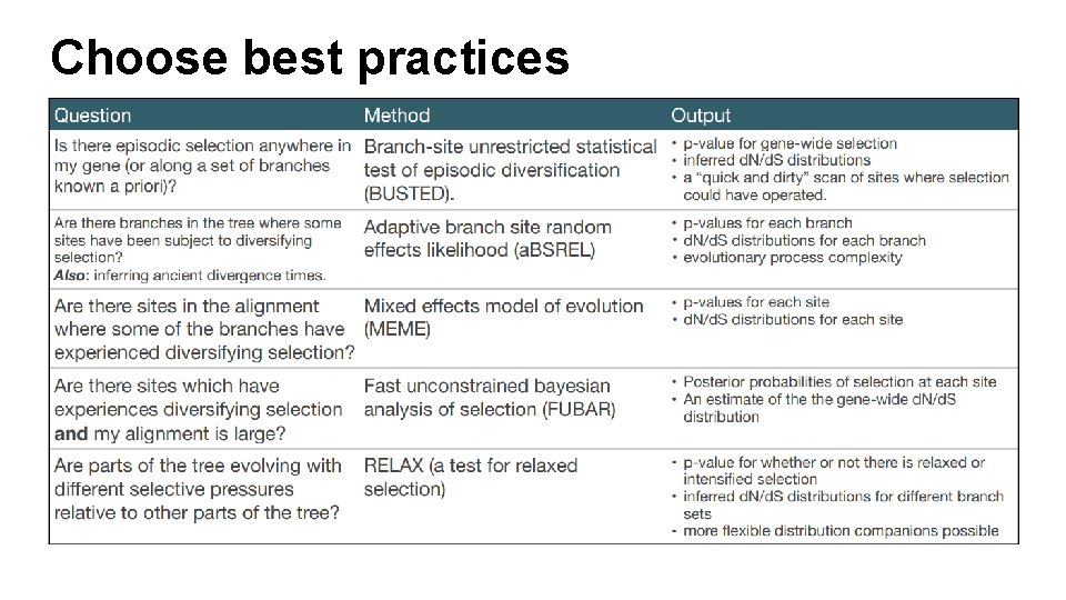
Choose best practices

Visit Datamonkeyhttp: //test. datamonkey. org/

Thank s！