Quality Control Chapter 5 Control Charts for Variables

Quality Control Chapter 5 - Control Charts for Variables 1

Outline q. The Control Chart Techniques q. State of Introduction q. Control q. Specifications q. Process Capability q. Six Sigma q. Different Control Charts 2

Learning Objectives (1/3) When you have completed this chapter you should: q. Know the three categories of variation and their sources. q. Understand the concept of the control chart method. q. Know the purpose of variable control charts. q. Know how to select the quality characteristics, the rational subgroup and the method of taking 3

Learning Objectives (2/3) When you have completed this chapter you should: q. Be able to calculate the central value, trial control limits and the revised control limits for Xbar and R chart. q. Be able to explain what is meant by a process in control and the various out-of-control patterns. q. Know the difference between individual measurements and averages; control limits and specifications. 4

Learning Objectives (3/3) When you have completed this chapter you should: q. Know the different situations between the process spread and specifications and what can be done to correct the undesirable situation. q. Be able to calculate process capability. q. Know the statistical meaning of 6σ 5

Variation (1/8) The variation concept is a law of nature in that no two natural items in any category are the same.

Variation (2/8) q. The variation may be quite large and easily noticeable q. The variation may be very small. It may appear that items are identical; however, precision instruments will show difference q. The ability to measure variation is necessary before it can be controlled

Variation (3/8) There are three categories of variation in piece part production: 1. Within-piece variation: Surface 2. Piece-to-piece variation: Among pieces produced at the same time 3. Time-to-time variation: Difference in product produced at different times of the day

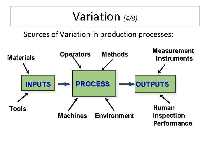
Variation (4/8) Sources of Variation in production processes: Materials INPUTS Tools Operators Methods PROCESS Machines Environment Measurement Instruments OUTPUTS Human Inspection Performance

Variation (5/8) Sources of variation are: 1. Equipment: 1. Toolwear 2. Machine vibration 3. Electrical fluctuations etc. 2. Material 1. Tensile strength 2. Ductility 3. Thickness 4. Porosity etc.

Variation (6/8) Sources of variation are: 3. Environment 1. Temperature 2. Light 3. Radiation 4. Humidity etc. 4. Operator 1. Personal problem 2. Physical problem etc.

Variation (7/8) There is also a reported variation which is due to the inspection activity. Variation due to inspection should account for one tenth of the four other sources of variation.

Variation (8/8) Variation may be due to chance causes (random causes) or assignable causes. When only chance causes are present, then the process is said to be in a state of statistical control. The process is stable and predictable.

Control Charts (1/2) q. Variable data q x-bar and R-charts q x-bar and s-charts q Charts for individuals (x-charts) q. Attribute data q For “defectives” (p-chart, np-chart) q For “defects” (c-chart, u-chart)

Control Charts (2/2) Continuous Numerical Data Control Charts Categorical or Discrete Numerical Data Variables Charts R Chart X Chart Attributes Charts P Chart C Chart 15

Control Charts for Variables The control chart for variables is a means of visualizing the variations that occur in the central tendency and the mean of a set of observations. It shows whether or not a process is in a stable state.

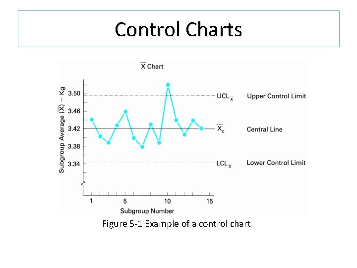
Control Charts Figure 5 -1 Example of a control chart

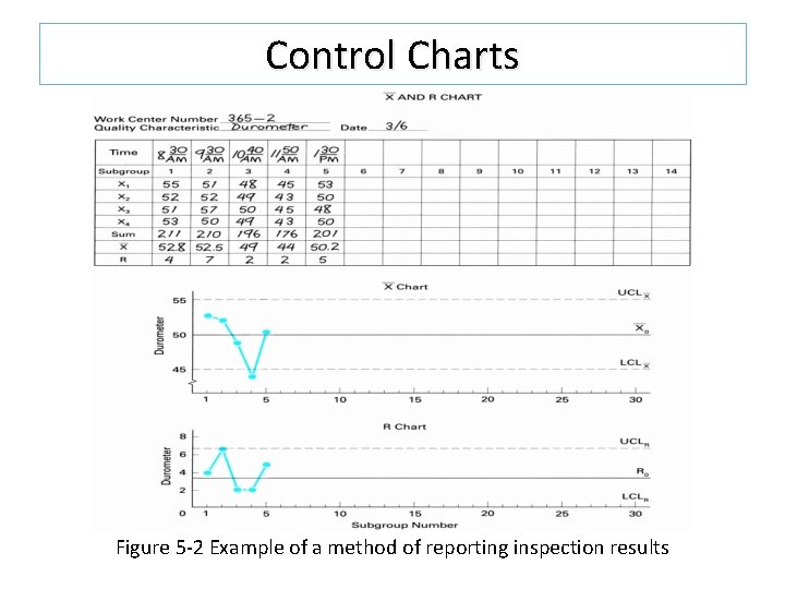
Control Charts Figure 5 -2 Example of a method of reporting inspection results

Variable Control Charts The objectives of the variable control charts are: 1. For quality improvement 2. To determine the process capability 3. For decisions regarding product specifications 4. For current decisions on the production process 5. For current decisions on recently produced items

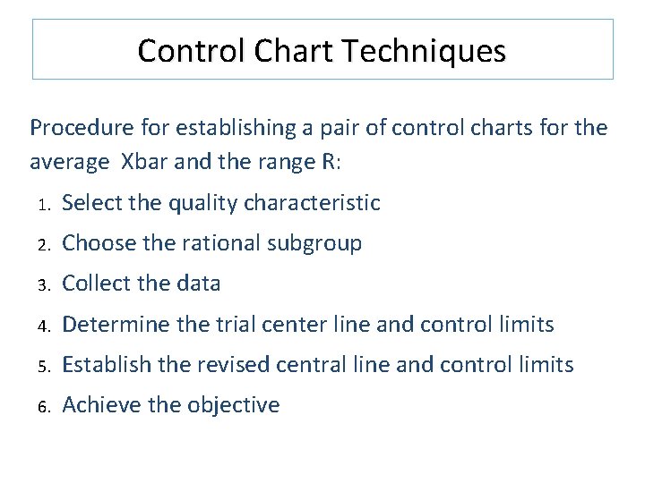
Control Chart Techniques Procedure for establishing a pair of control charts for the average Xbar and the range R: 1. Select the quality characteristic 2. Choose the rational subgroup 3. Collect the data 4. Determine the trial center line and control limits 5. Establish the revised central line and control limits 6. Achieve the objective

Quality Characteristic The Quality characteristic must be measurable. It can expressed in terms of the seven basic units: 1. Length 2. Mass 3. Time 4. Electrical current 5. Temperature 6. Substance 7. Luminosity as appropriate.

Rational Subgroup (1/3) A rational subgroup is one in which the variation within a group is due only to chance causes. Within-subgroup variation is used to determine the control limits. Variation between subgroups is used to evaluate longterm stability.

Rational Subgroup (2/3) There are two schemes for selecting the subgroup samples: 1. Select subgroup samples from product or service produced at one instant of time or as close to that instant as possible---instant-time method 2. Select from product or service produced over a period of time that is representative of all the products or services---period-of-time method

Rational Subgroup (3/3) The first scheme will have a minimum variation within a subgroup. The second scheme will have a minimum variation among subgroups. The first scheme is the most commonly used since it provides a particular time reference for determining assignable causes. The second scheme provides better overall results and will provide a more accurate picture of the quality.

Subgroup Size q As the subgroup size increases, the control limits become closer to the central value, which make the control chart more sensitive to small variations in the process average q As the subgroup size increases, the inspection cost per subgroup increases q When destructive testing is used and the item is expensive, a small subgroup size is required

Subgroup Size q From a statistical basis a distribution of subgroup averages are nearly normal for groups of 4 or more even when samples are taken from a non-normal distribution q When a subgroup size of 10 or more is used, the s chart should be used instead of the R chart. q See Table 5 -1 for sample sizes

Data Collection Data collection can be accomplished using the type of figure shown in Figure 5 -2. It can also be collected using the method in Table 5 -2. It is necessary to collect a minimum of 25 subgroups of data. A run chart can be used to analyze the data in the development stage of a product or prior to a state of statistical control

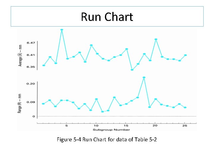
Run Chart Figure 5 -4 Run Chart for data of Table 5 -2

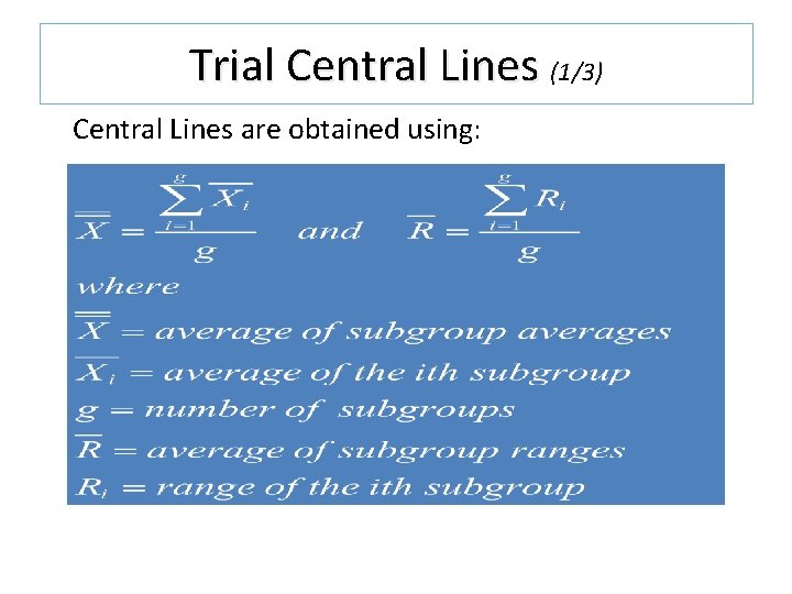
Trial Central Lines (1/3) Central Lines are obtained using:

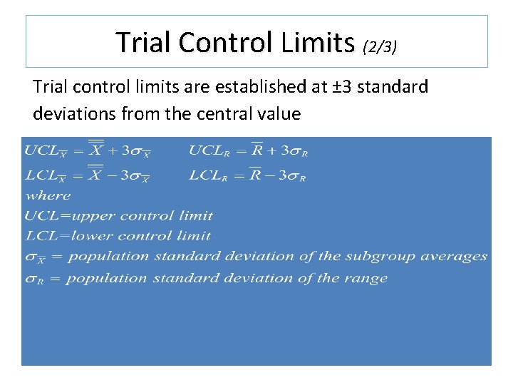
Trial Control Limits (2/3) Trial control limits are established at ± 3 standard deviations from the central value

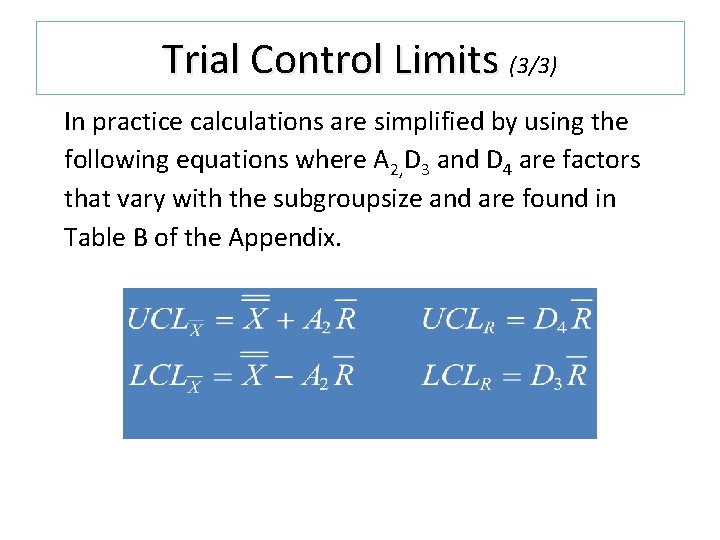
Trial Control Limits (3/3) In practice calculations are simplified by using the following equations where A 2, D 3 and D 4 are factors that vary with the subgroupsize and are found in Table B of the Appendix.

Trial Control Limits Figure 5 -5 Xbar and R chart for preliminary data with trial control limits

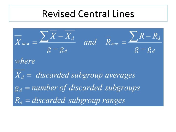
Revised Central Lines

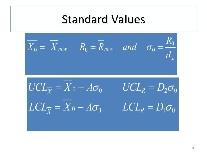
Standard Values 34

Figure 5 -6 Trial control limits and revised control limits for Xbar and R charts

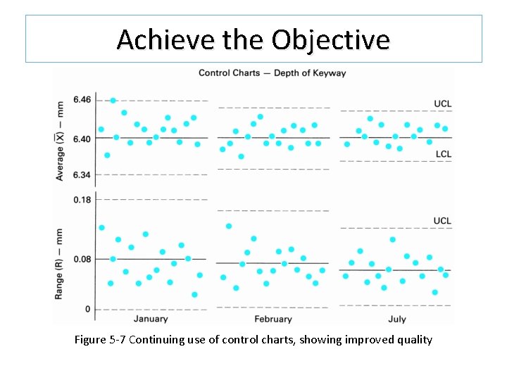
Achieve the Objective Figure 5 -7 Continuing use of control charts, showing improved quality

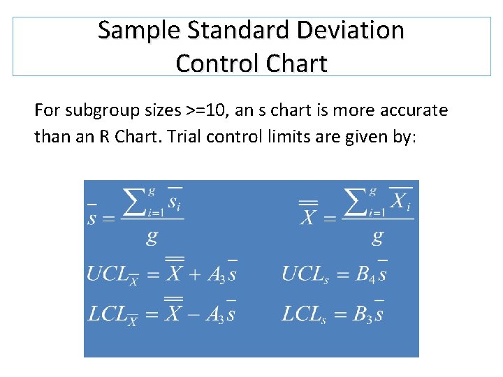
Sample Standard Deviation Control Chart For subgroup sizes >=10, an s chart is more accurate than an R Chart. Trial control limits are given by:

State of Control (1/8) Process in Control q When special causes have been eliminated from the process to the extent that the points plotted on the control chart remain within the control limits, the process is in a state of control q When a process is in control, there occurs a natural pattern of variation

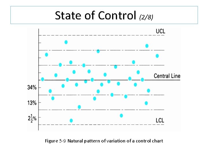
State of Control (2/8) Figure 5 -9 Natural pattern of variation of a control chart

State of Control (3/8) Types of errors: q Type I, occurs when looking for a special cause of variation when in reality a common cause is present q Type II, occurs when assuming that a common cause of variation is present when in reality there is a special cause

State of Control(4/8) When the process is in control: 1. Individual units of the product or service will be more uniform 2. Since the product is more uniform, fewer samples are needed to judge the quality 3. The process capability or spread of the process is easily attained from 6σ 4. Trouble can be anticipated before it occurs

State of Control (5/8) When the process is in control: 5. The % of product that falls within any pair of values is more predictable 6. It allows the consumer to use the producer’s data 7. It is an indication that the operator is performing satisfactorily

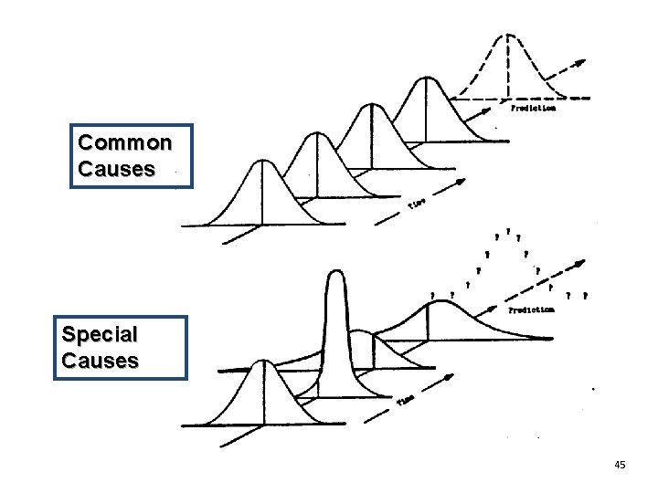
Common Causes Special Causes 45

State of Control (6/8) Figure 5 -11 Frequency Distribution of subgroup averages with control limits

State of Control (7/8) When a point (subgroup value) falls outside its control limits, the process is out of control. Out of control means a change in the process due to a special cause. A process can also be considered out of control even when the points fall inside the 3σ limits

State of Control (8/8) q It is not natural for seven or more consecutive points to be above or below the central line. q Also when 10 out of 11 points or 12 out of 14 points are located on one side of the central line, it is unnatural. q Six points in a row are steadily increasing or decreasing indicate an out of control situation

Out-of-Control Condition 1. 2. 3. 4. 5. Change or jump in level. Trend or steady change in level Recurring cycles Two populations (also called mixture) Mistakes

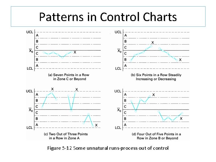
Patterns in Control Charts Figure 5 -12 Some unnatural runs-process out of control

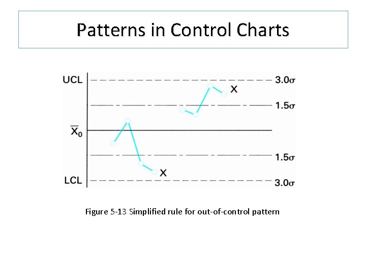
Patterns in Control Charts Figure 5 -13 Simplified rule for out-of-control pattern

Out-of-Control Patterns Change or jump in level Trend or steady change in level Recurring cycles Two populations

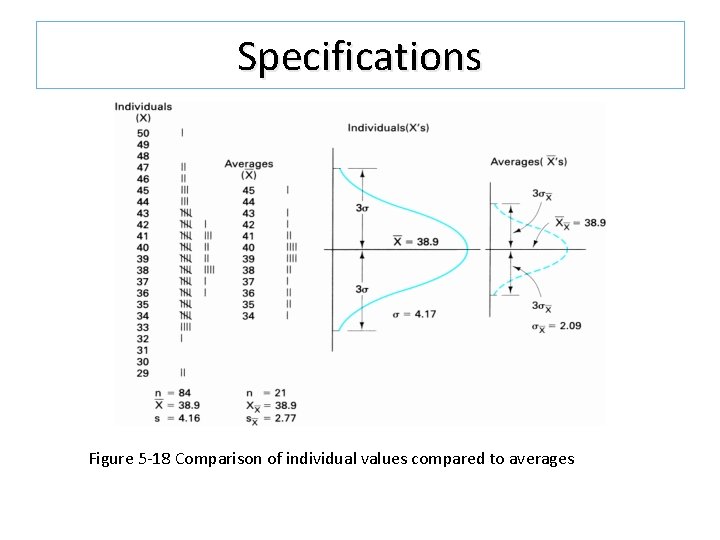
Specifications Figure 5 -18 Comparison of individual values compared to averages

Specifications Calculations of the average for both the individual values and for the subgroup averages are the same. However the sample standard deviation is different.

Central Limit Theorem If the population from which samples are taken is not normal, the distribution of sample averages will tend toward normality provided that the sample size, n, is at least 4. This tendency gets better and better as the sample size gets larger. The standardized normal can be used for the distribution averages with the modification.

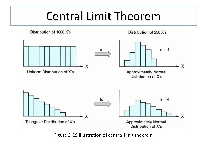
Central Limit Theorem Figure 5 -19 Illustration of central limit theorem

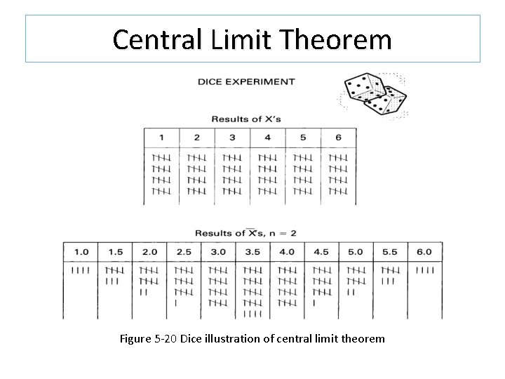
Central Limit Theorem Figure 5 -20 Dice illustration of central limit theorem

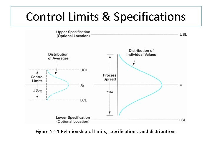
Control Limits & Specifications Figure 5 -21 Relationship of limits, specifications, and distributions

Control Limits & Specifications q The control limits are established as a function of the average q Specifications are the permissible variation in the size of the part and are, therefore, for individual values q The specifications or tolerance limits are established by design engineers to meet a particular function

Process Capability & Tolerance(1/5) q The process spread will be referred to as the process capability and is equal to 6σ q The difference between specifications is called the tolerance q When the tolerance is established by the design engineer without regard to the spread of the process, undesirable situations can result

Process Capability & Tolerance(2/5) Three situations are possible: q Case I: When the process capability is less than the tolerance 6σ<USL-LSL q Case II: When the process capability is equal to the tolerance 6σ=USL-LSL q Case III: When the process capability is greater than the tolerance 6σ >USL-LSL

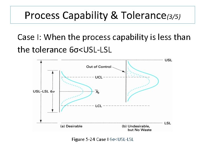
Process Capability & Tolerance(3/5) Case I: When the process capability is less than the tolerance 6σ<USL-LSL Figure 5 -24 Case I 6σ<USL-LSL

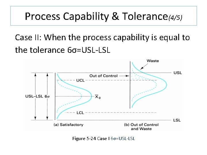
Process Capability & Tolerance(4/5) Case II: When the process capability is equal to the tolerance 6σ=USL-LSL Figure 5 -24 Case I 6σ=USL-LSL

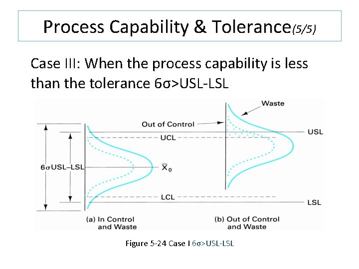
Process Capability & Tolerance(5/5) Case III: When the process capability is less than the tolerance 6σ>USL-LSL Figure 5 -24 Case I 6σ>USL-LSL

Process Capability(1/3) q The range over which the natural variation of a process occurs as determined by the system of common causes q Measured by the proportion of output that can be produced within design specifications 63

Process Capability(2/3) This following method of calculating the process capability assumes that the process is stable or in statistical control: q Take 25 (g) subgroups of size 4 for a total of 100 measurements q Calculate the range, R, for each subgroup q Calculate the average range, RBar= ΣR/g q Calculate the estimate of the population standard deviation q Process capability will equal 6σ0

Process Capability(3/3) The process capability can also be obtained by using the standard deviation: q Take 25 (g) subgroups of size 4 for a total of 100 measurements q Calculate the sample standard deviation, s, for each subgroup q Calculate the average sample standard deviation, sbar = Σs/g q Calculate the estimate of the population standard deviation q. Process capability will equal 6σo

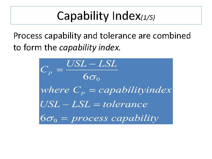
Capability Index(1/5) Process capability and tolerance are combined to form the capability index.

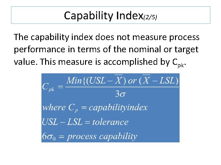
Capability Index(2/5) The capability index does not measure process performance in terms of the nominal or target value. This measure is accomplished by Cpk.

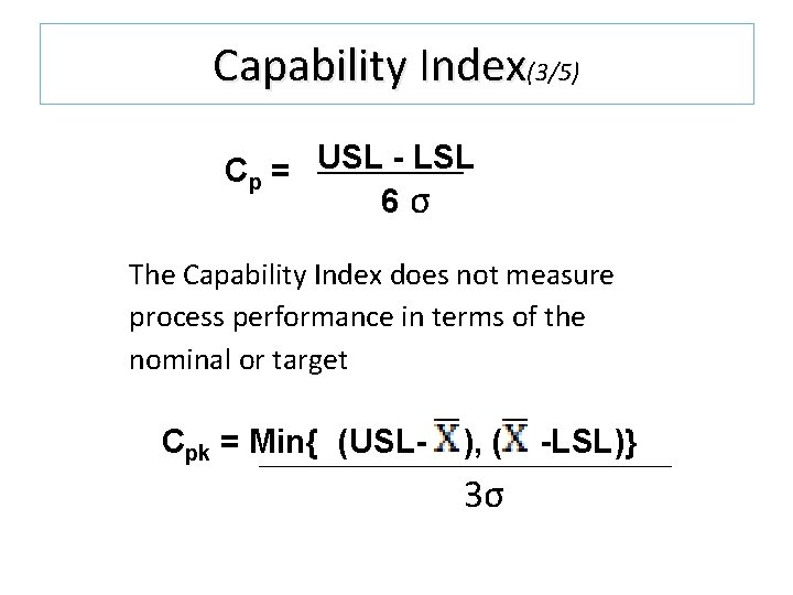
Capability Index(3/5) Cp = USL - LSL 6σ The Capability Index does not measure process performance in terms of the nominal or target Cpk = Min{ (USL- ), ( 3σ -LSL)}

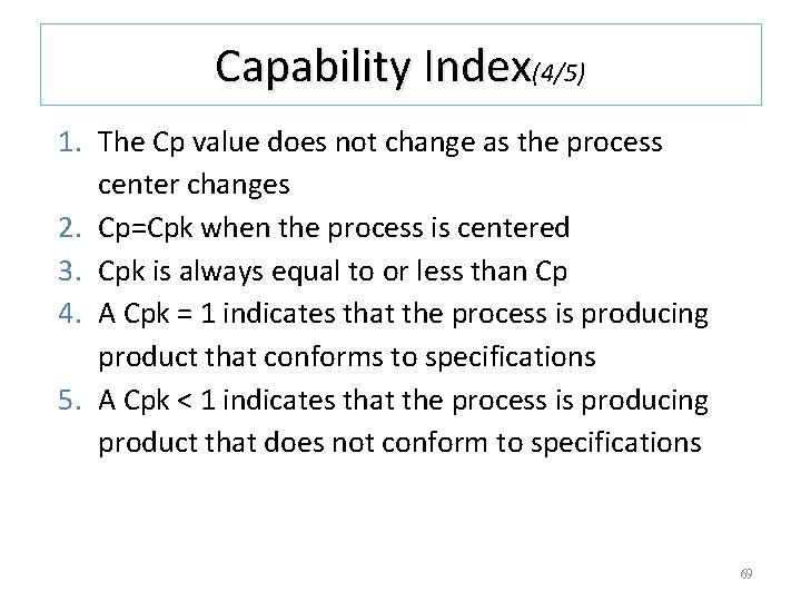
Capability Index(4/5) 1. The Cp value does not change as the process center changes 2. Cp=Cpk when the process is centered 3. Cpk is always equal to or less than Cp 4. A Cpk = 1 indicates that the process is producing product that conforms to specifications 5. A Cpk < 1 indicates that the process is producing product that does not conform to specifications 69

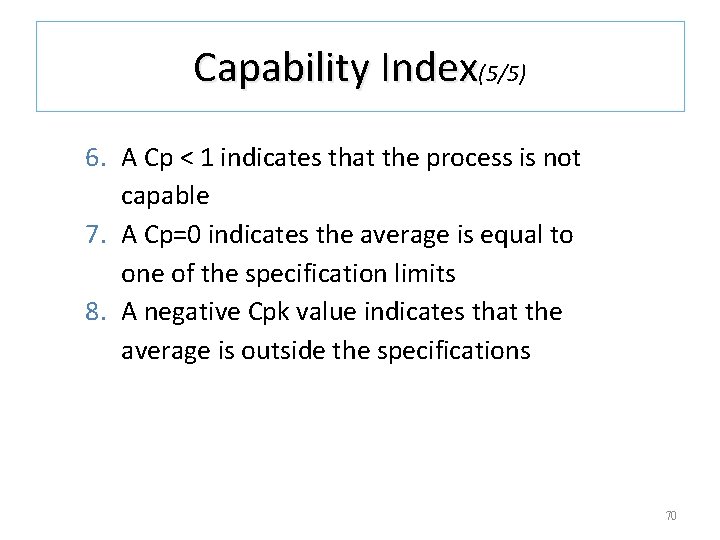
Capability Index(5/5) 6. A Cp < 1 indicates that the process is not capable 7. A Cp=0 indicates the average is equal to one of the specification limits 8. A negative Cpk value indicates that the average is outside the specifications 70

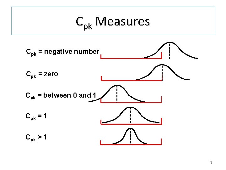
Cpk Measures Cpk = negative number Cpk = zero Cpk = between 0 and 1 Cpk = 1 Cpk > 1 71

Six Sigma is both a quality management philosophy and a methodology that focuses on reducing variation, measuring defects, and improving quality of products, processes and services. 72

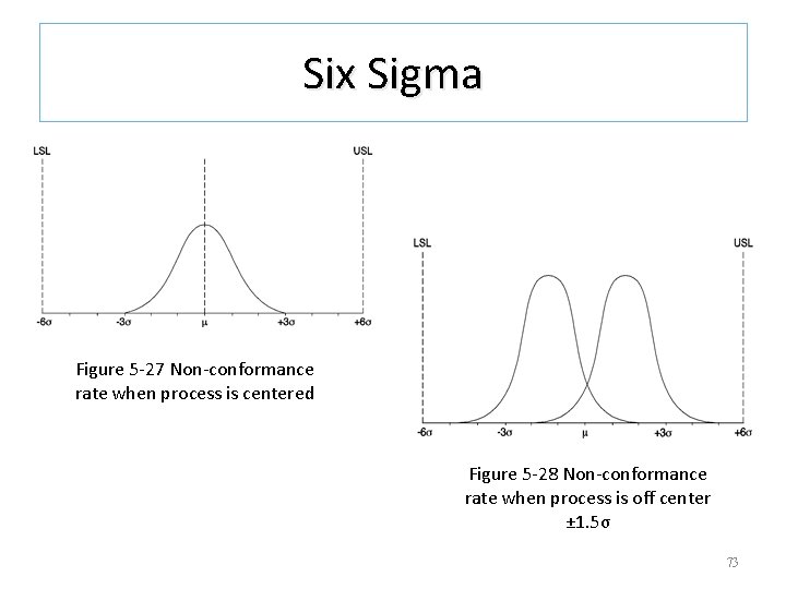
Six Sigma Figure 5 -27 Non-conformance rate when process is centered Figure 5 -28 Non-conformance rate when process is off center ± 1. 5σ 73

Different Control Charts for Better Operator Understanding: 1. Placing individual values on the chart: This technique plots both the individual values and the subgroup average. Not recommended since it does not provide much information. 2. Chart for subgroup sums: This technique plots the subgroup sum, ΣX, rather than the group average, Xbar.

Different Control Charts for Variable Subgroup Size: Used when the sample size is not the same q Different control limits for each subgroup q As n increases, limits become narrower q As n decreases, limits become wider apart q Difficult to interpret and explain q To be avoided

Different Control Charts Chart for Trends: Used when the plotted points have an upward or downward trend that can be attributed to an unnatural pattern of variation or a natural pattern such as tool wear. The central line is on a slope, therefore its equation must be determined.

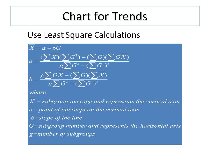
Chart for Trends Use Least Square Calculations

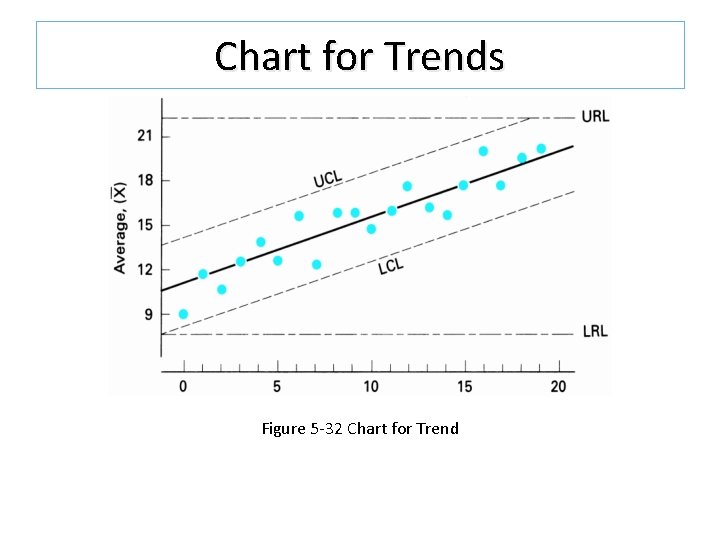
Chart for Trends Figure 5 -32 Chart for Trend

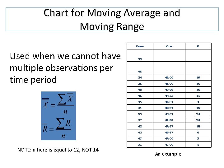
Chart for Moving Average and Moving Range Value Used when we cannot have multiple observations per time period NOTE: n here is equal to 12, NOT 14 Xbar R 54 48. 00 10 38 46. 00 16 49 47. 00 16 46 44. 33 11 45 46. 67 4 31 40. 67 15 55 43. 67 24 37 41. 00 24 42 44. 67 18 43 40. 67 6 47 44. 00 5 51 47. 00 8 44 46 An example

Chart for Moving Average and Moving Range Extreme readings have a greater effect than in conventional charts. An extreme value is used several times in the calculations, the number of times depends on the averaging period. 80

Chart for Median and Range This is a simplified variable control chart. q Minimizes calculations q Easier to understand q Can be easily maintained by operators q Recommended to use a subgroup of 3, then all data is used. 81

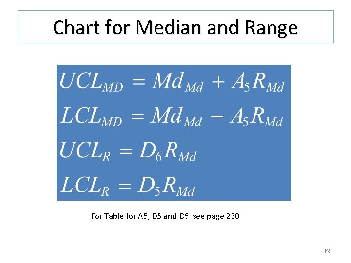
Chart for Median and Range For Table for A 5, D 5 and D 6 see page 230 82

Chart for Individual values Used when only one measurement is taken on quality characteristic q Too expensive q Time consuming q Destructive q Very few items 83

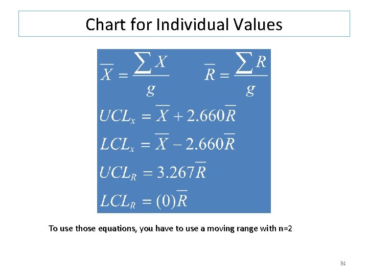
Chart for Individual Values To use those equations, you have to use a moving range with n=2 84

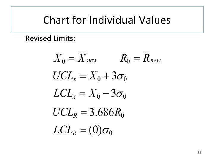
Chart for Individual Values Revised Limits: 85

Charts with Non-Acceptance Limits Non-Acceptance limits have the same Relationship to averages as specifications have to individual values. Control Limits tell what the process is capable of doing, and reject limits tell when the product is conforming to specifications. 86

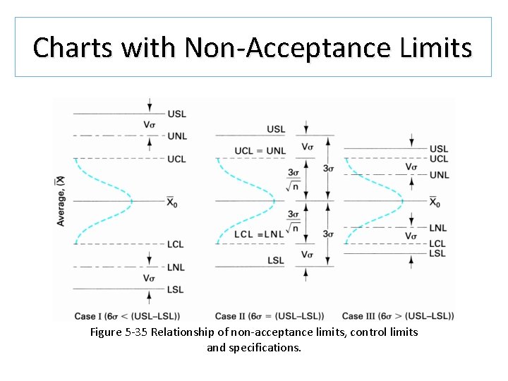
Charts with Non-Acceptance Limits Figure 5 -35 Relationship of non-acceptance limits, control limits and specifications.