Qualitative Response Model probit model logit model probit

Qualitative Response Model 質的反応モデル
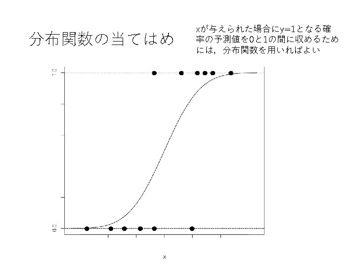

probit model, logit model •
 •")
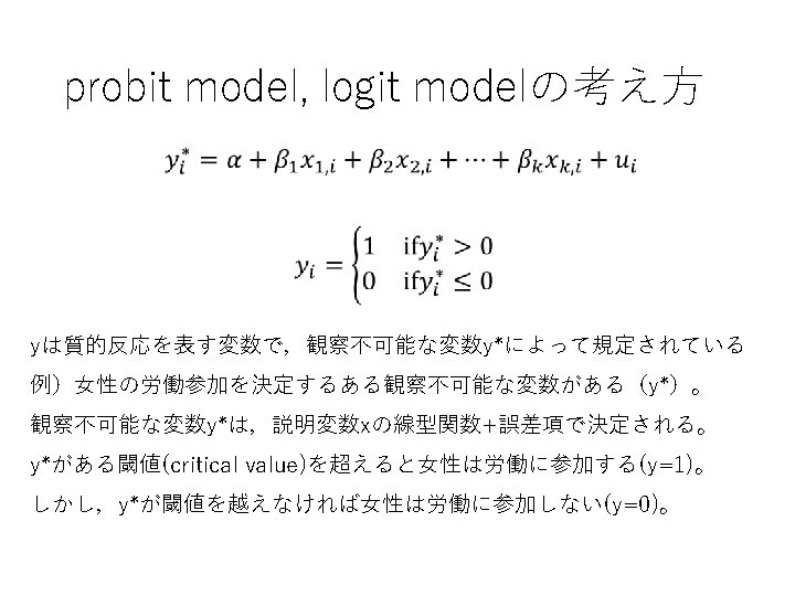
probit model, logit modelの考え方(続き) •
という関数を用いる probit : glm(formula, family=binomial(link=“probit”)) logit")
probit and logit model : R • glm( )という関数を用いる probit : glm(formula, family=binomial(link=“probit”)) logit : glm(formula, family=binomial(link=“logit”)) • object <- glm( ) で結果を保存し,summary(object) で結果の 要約を出力 例) inlf_probit <- glm(inlf ~ nwifeinc + educ + exper + age + kidslt 6 + kidsge 6 , family=binomial(link=“probit”)) summary(inlf_probit)
 •")
probit and logit model : R (2) •
 Call: glm(formula = inlf ~ nwifeinc + educ + exper")
probit model: Rの結果(mroz. xls) Call: glm(formula = inlf ~ nwifeinc + educ + exper + age + kidslt 6 + kidsge 6, family = binomial(link = "probit")) Coefficients: Estimate Std. Error z value Pr(>|z|) (Intercept) 0. 579574 0. 495537 1. 170 0. 2422 nwifeinc -0. 011565 0. 004858 -2. 380 0. 0173 * educ 0. 133690 0. 025254 5. 294 1. 20 e-07 *** exper 0. 070217 0. 007693 9. 127 < 2 e-16 *** age -0. 055555 0. 008305 -6. 689 2. 24 e-11 *** kidslt 6 -0. 874290 0. 117359 -7. 450 9. 35 e-14 *** kidsge 6 0. 034546 0. 043376 0. 796 0. 4258 --Signif. codes: 0 ‘***’ 0. 001 ‘**’ 0. 01 ‘*’ 0. 05 ‘. ’ 0. 1 ‘ ’ 1 Null deviance: 1029. 75 on 752 degrees of freedom Residual deviance: 812. 44 on 746 degrees of freedom AIC: 826. 44
 glm(formula = inlf ~ nwifeinc + educ +")
logit model: Rの結果 ( mroz. xls) glm(formula = inlf ~ nwifeinc + educ + exper + age + kidslt 6 + kidsge 6, family = binomial(link = "logit")) Coefficients: Estimate Std. Error z value Pr(>|z|) (Intercept) 0. 837909 0. 840933 0. 996 0. 3191 nwifeinc -0. 020216 0. 008264 -2. 446 0. 0144 * educ 0. 226977 0. 043295 5. 243 1. 58 e-07 *** exper 0. 119746 0. 013626 8. 788 < 2 e-16 *** age -0. 091088 0. 014321 -6. 361 2. 01 e-10 *** kidslt 6 -1. 439393 0. 201498 -7. 143 9. 10 e-13 *** kidsge 6 0. 058174 0. 073380 0. 793 0. 4279 --Signif. codes: 0 ‘***’ 0. 001 ‘**’ 0. 01 ‘*’ 0. 05 ‘. ’ 0. 1 ‘ ’ 1 Null deviance: 1029. 75 Residual deviance: 812. 29 AIC: 826. 29 on 752 on 746 degrees of freedom

probit and logit model : Stata Probit: メニューから Statistics /Binary outcomes /Probit regression 右の画面で,変数を選択 Logit: メニューから Statistics /Binary outcomes /Logistic regression defaultでodds ratioが出力 される 回帰係数を出力するために はReportingタブを選択し, Report estimated coefficients を選択

probit and logit model : Eviews menu から Quick Estimate equation を選択 右の画面Estimation settings で method にBINARYを選択 specificationに Binary estimation method というoptionが表れる ので,Probit または Logit を選択する

Probit model: Eviews

係数の比較 ols coef probit s. e. coef logit s. e. coef s. e. C 0. 707 0. 150 0. 580 0. 496 0. 838 0. 841 NWIFEINC -0. 003 0. 001 -0. 012 0. 005 -0. 020 0. 008 EDUC 0. 040 0. 007 0. 134 0. 025 0. 227 0. 043 EXPER 0. 023 0. 002 0. 070 0. 008 0. 120 0. 014 AGE -0. 018 0. 002 -0. 056 0. 008 -0. 091 0. 014 KIDSLT 6 -0. 272 0. 034 -0. 874 0. 118 -1. 439 0. 201 KIDSGE 6 0. 013 0. 035 0. 043 0. 058 0. 073

係数の意味: marginal effects •
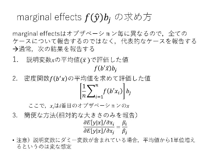
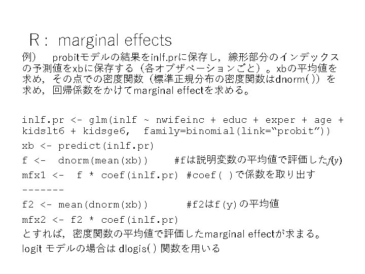

marginal effects •

Stata: marginal effects probit, logit model 推計後, メ ニューから Statistics /Post estimation で右の画面 Marginal effects of all covariates から Population averaged… またはAt sample meansを選択 sample mean 前ページ 1 の方法 population averaged. . 前 ページ 2の方法
を選択 右の画面 Series to ForecastでIndexを選択し, Forecast nameに保存する変数名を 指定(右図ではinlff)")
Eviews: marginal effects estimation outputのmenuから Proc/Forecast(Fitted Probability/Index)を選択 右の画面 Series to ForecastでIndexを選択し, Forecast nameに保存する変数名を 指定(右図ではinlff) 平均値 @mean( ) 標準正規分布の密度関数 @dnorm( ) 係数b @coefs (@coefには最後に行った回帰分析 の係数が保存されている)
 Inlffにb’xが保存されているとして • 説明変数の平均値で評価したmarginal effects コマンドラインで次のようにタイプする vector mfx 1 = @dnorm(@mean(inlff)")
Eviews : marginal effects(2) Inlffにb’xが保存されているとして • 説明変数の平均値で評価したmarginal effects コマンドラインで次のようにタイプする vector mfx 1 = @dnorm(@mean(inlff) )* @coefs • 密度関数の平均値で評価する方法 series f = @dnorm(inlff) vector mfx 2 = @mean(f) * @coefs mfx 1, mfx 2にmarginal effectsが入る logit modelの場合の密度関数は @dlogistic( )を用いる
 regression •")
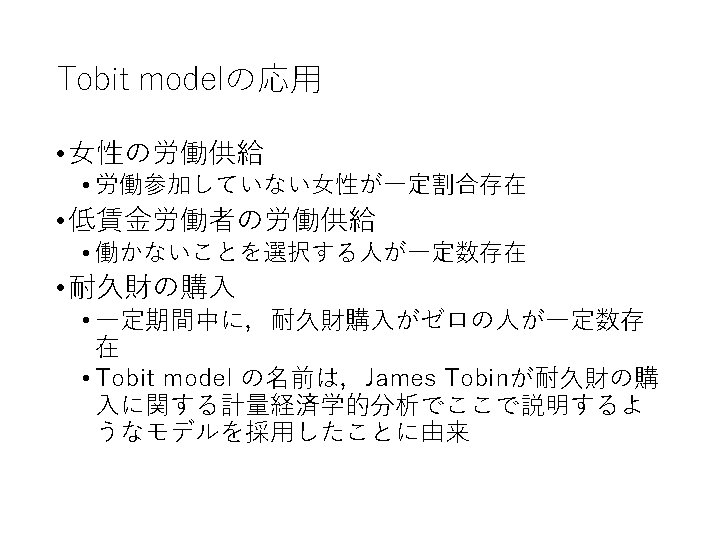
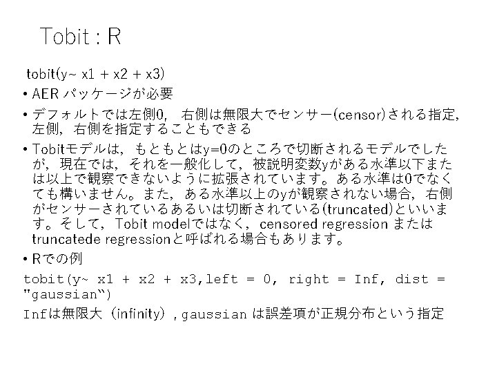
Tobit model censored (truncated) regression •

Tobit model の当てはめ y OLSの当てはめ x y*とxの関係 Tobit model

Tobit model の想定 •

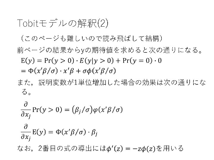
Tobit model の解釈 • inverse Mills ratio

Tobit: Rの出力画面 データ: mroz. xls 被説明変数: hours Coefficients: Estimate Std. Error z value P r(>|z|) (Intercept) 965. 30530 446. 43614 2. 162 0. 030599 * nwifeinc -8. 81424 4. 45910 -1. 977 0. 048077 * educ 80. 64561 21. 58324 3. 736 0. 000187 *** exper 131. 56430 17. 27939 7. 614 2. 66 e-14 *** expersq -1. 86416 0. 53766 -3. 467 0. 000526 *** age -54. 40501 7. 41850 -7. 334 2. 24 e-13 *** kidslt 6 -894. 02174 111. 87804 -7. 991 1. 34 e-15 *** kidsge 6 -16. 21800 38. 64139 -0. 420 0. 674701 Log(scale) 7. 02289 0. 03706 189. 514 < 2 e-16 *** --Signif. codes: 0 ‘***’ 0. 001 ‘**’ 0. 01 ‘*’ 0. 05 ‘. ’ 0. 1 ‘ ’ 1 Scale: 1122 Gaussian distribution Number of Newton-Raphson Iterations: 4 Log-likelihood: -3819 on 9 Df Wald-statistic: 253. 9 on 7 Df, p-value: < 2. 22 e-16 sの推計値

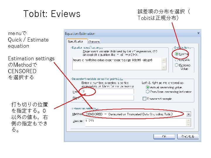
Tobit : Stata メニューから Statistics > Linear models and related > Censored regression > Tobit regression 右の画面で 被説明変数,説明変数 の指定 specify censoring limit の指定 この場合,hoursは左側 0でセンサーされている ので,そのように指定 する
 = 271. 59 Prob > chi 2 =")
Tobit: Stata の出力画面 LR chi 2(7) = 271. 59 Prob > chi 2 = 0. 0000 Log likelihood = -3819. 0946 Pseudo R 2 = 0. 0343 --------------------------------------hours | Coef. Std. Err. t P>|t| [95% Conf. Interval] ------+--------------------------------nwifeinc | -8. 814226 4. 459089 -1. 98 0. 048 -17. 56808 -. 0603705 educ | 80. 64541 21. 58318 3. 74 0. 000 38. 27441 123. 0164 exper | 131. 564 17. 27935 7. 61 0. 000 97. 64211 165. 486 expersq | -1. 864153. 5376606 -3. 47. 001 -2. 919661 -. 8086455 age | -54. 40491 7. 418483 -7. 33 0. 000 -68. 9685 -39. 84133 kidslt 6 | -894. 0202 111. 8777 -7. 99 0. 000 -1113. 653 -674. 3875 kidsge 6 | -16. 21806 38. 6413 -0. 42 0. 675 -92. 07668 59. 64057 _cons | 965. 3068 446. 4351 2. 16 0. 031 88. 88828 1841. 725 ------+--------------------------------var(e. hours)| 1258927 93304. 48 1088458 1456093 -------------------------------------- s 2の推定値

E-ViewsでのTobit modelの推定 sの推計値

Tobit model とOLSの比較 Dependent var hours Tobit OLS Coef s. e. C E-Viewsでの出 力の比較 965. 31 446. 44 1330. 48 270. 78 NWIFEINC -8. 81 4. 46 -3. 45 2. 54 EDUC 80. 65 21. 58 28. 76 12. 95 EXPER 131. 56 17. 28 65. 67 9. 96 -1. 86 0. 54 -0. 70 0. 32 -54. 41 7. 42 -30. 51 4. 36 KIDSLT 6 -894. 02 111. 88 -442. 09 58. 85 KIDSGE 6 -16. 22 38. 64 -32. 78 23. 18 s 1122. 02 EXPERSQ AGE 750. 179 Tobitの場合,xj の 1単位の増加 がy*ではなくy に与える影響を みるためには, x’b/s を計算し, その累積分布を 計算する必要あ り。
- Slides: 40